Fundamentals of linear mixed models
Topics: Linear models review; Fixed effects vs. random effects
- Welcome!
- Housekeeping
- Outline for today
- Linear models review
- Adding a random effect to the model
- Generalities on mixed models
- Applied example
- Discussions
- Summary
- What’s next
Welcome!
- About us: Josefina and Claudio.
- About you.
- Frequent responses to the registration survey.
- Some knowledge of the existence of mixed effects models.
- Mostly life sciences - often heteroscedasticity (tomorrow) and dependent observations (this workshop)!
Housekeeping
- We will have relatively low proportion of R code in this workshop. Instead, we will focus on the understanding of the components of mixed-effects models. Questions/concerns via e-mail are encouraged.
- Emphasis on modeling and figuring out what mixed-effects models actually do.
- The statistical notation we will use throughout this workshop is presented here.
- DON’T PANIC when you see all the math notation and matrices. We will go slowly together. It is also not expected that you walk out of this workshop as a math notation wizard!
Part 1. Fundamentals of linear mixed models
Review of linear models & basic concepts of linear mixed models
Part 2. Modeling data generated by designed experiments
Part 3. Generalized linear mixed models (aka non-normal response) applied to designed experiments
Outline for today
- Review of linear models: begin with a refresher on linear models (all fixed-effects), then introduce mixed-effects models by incorporating an additional assumption.
- The variance-covariance matrix: the information of the random effects is stored in the variance-covariance matrix!
- Fixed effects vs. random effects: where/how is the information from each type of effect captured?
- Application: practical implications of these concepts when fitting a model to your data.
Linear models review
The quadratic regression is a linear model, too
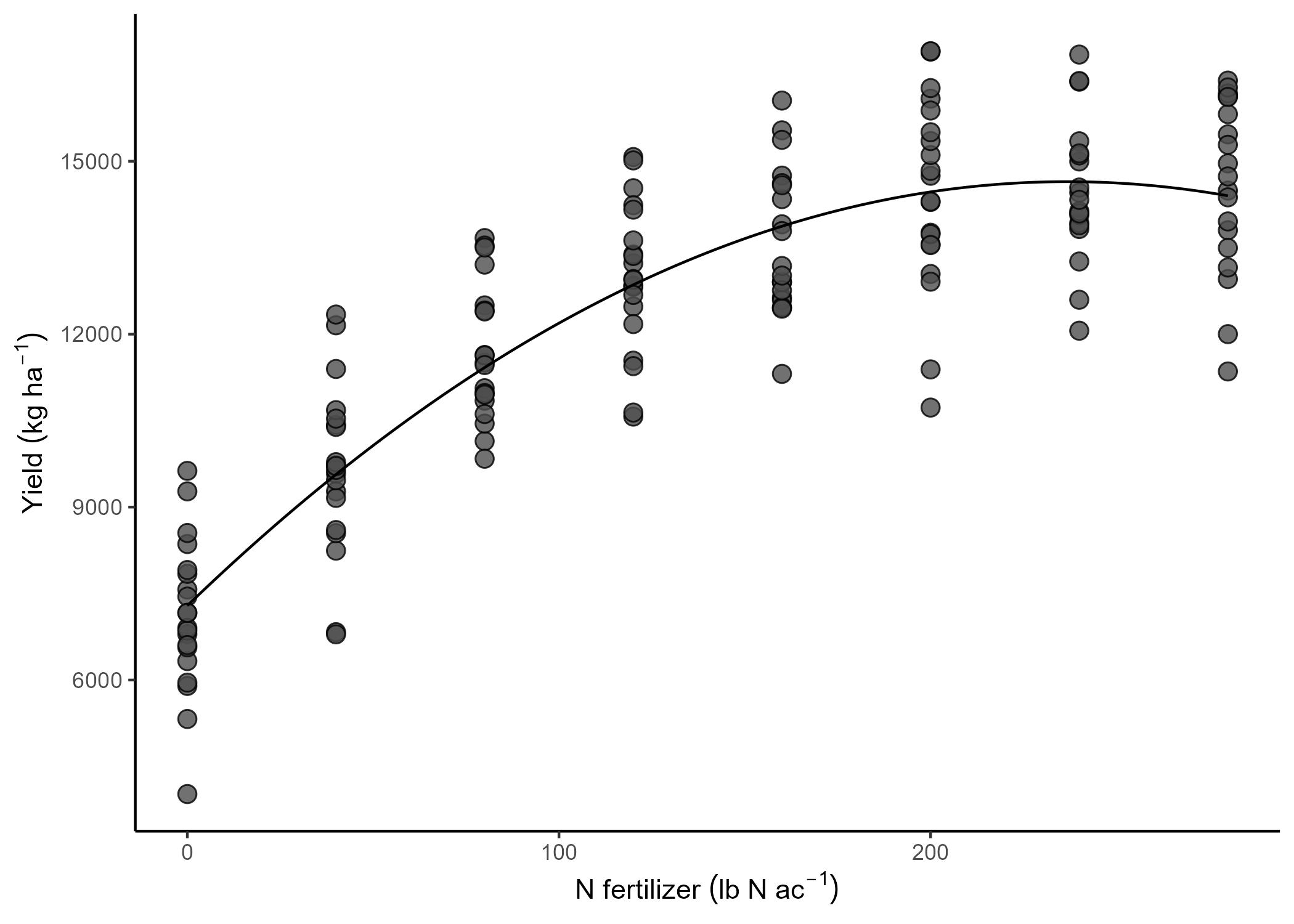
One of the most popular linear models is the intercept-and-slope model (sometimes also called linear regression), often used to describe the (linear) relationship between two quantitative variables. Quadratic regression is also a linear model, and it’s often used to describe relationship between two quantitative variables when it’s not exactly linear, but has some type of curvature.
Most of us learned a way of writing out the statistical model called “model equation form”. For a quantitative predictor \(x\), the model equation form is
\[y_{i} = \beta_0 + x_{i} \beta_1 + x_{i}^2 \beta_2 + \varepsilon_{i}, \\ \varepsilon_i \sim N(0, \sigma^2),\]where \(y_{i}\) is the observed value for the \(i\)th observation, \(\beta_0\) is the intercept (i.e., the expected value of \(y\) when \(x=0\)), \(\beta_1\) is the linear component (i.e., the expected change in \(y_i\) with a unity increase in \(x\)), \(\beta_2\) is the quadratic component (i.e., the expected change in \(y_i\) with a unity increase in \(x^2\)), \(x_i\) is the predictor for the \(i\)th observation, and \(\varepsilon_{i}\) is the difference between the observed value \(y\) and the expected value \(E(y_i) = \beta_0+x_i\beta_1+ x_{i}^2 \beta_2\) - that’s why we often call it “residual”. Typically, \(\boldsymbol{\beta} \equiv \begin{bmatrix} \beta_0 \\ \beta_1 \\ \beta_2 \end{bmatrix}\) is estimated via maximum likelihood estimation. Also, when we assume a Normal distribution, maximum likelihood estimation yields the same point estimates as least squares estimation.
Let’s review the assumptions we make in this model (which is the default model in most software).
- Linearity
- Constant variance
- Independence
- Normality
Let’s review that simple model using distribution notation and matrix notation
There are other ways of writing out the statistical model above, besides the model equation form. Instead of focusing on the distribution of the residuals, we can focus on the distribution of the data \(y\):
\[y_{i} \sim N(\mu_i, \sigma^2), \\ \mu_i = \beta_0 + x_{i} \beta_1 + x_{i}^2 \beta_2.\]This type of notation is called “probability distribution form”. The probability distribution form makes it easier to switch to other distributions beyond the Normal (Part 3 of this workshop). We can further express this equation using vectors and matrices:
\[\mathbf{y} \sim N(\boldsymbol{\mu}, \Sigma), \\ \boldsymbol{\mu} = \boldsymbol{1} \beta_0 + \mathbf{x} \beta_1 = \mathbf{X}\boldsymbol{\beta},\]where \(n\) is the total number of observations, \(p\) is the total number of parameters, \(\mathbf{y}\) is an \(n \times 1\) vector containing all observations, \(\boldsymbol{\mu}\) is an \(n \times 1\) vector containing the expected values of said observations, \(\boldsymbol{\beta}\) is an \(p \times 1\) vector containing the (fixed) parameters, \(\mathbf{X}\) is an \(n \times p\) matrix containing the predictors, \(\Sigma\) is an \(n \times n\) matrix called variance-covariance matrix. Note: This type of notation is also convenient to think about how to prepare the data in your spreadsheet. One row per observation (rows in \(\mathbf{X}\)), one variable per column (columns in \(\mathbf{X}\)).
These expressions can be expanded into:
\[\begin{bmatrix}y_1 \\ y_2 \\ \vdots \\ y_n \end{bmatrix} \sim N \left( \begin{bmatrix}\mu_1 \\ \mu_2 \\ \vdots \\ \mu_n \end{bmatrix}, \begin{bmatrix} Cov(y_1, y_1) & Cov(y_1, y_2) & \dots & Cov(y_1, y_n) \\ Cov(y_2, y_1) & Cov(y_2, y_2) & \dots & Cov(y_2, y_n)\\ \vdots & \vdots & \ddots & \vdots \\ Cov(y_n, y_1) & Cov(y_n, y_2) & \dots & Cov(y_n, y_n) \end{bmatrix} \right),\]which is the same as
\[\begin{bmatrix}y_1 \\ y_2 \\ \vdots \\ y_n \end{bmatrix} \sim N \left( \begin{bmatrix}\mu_1 \\ \mu_2 \\ \vdots \\ \mu_n \end{bmatrix}, \begin{bmatrix} Var(y_1) & Cov(y_1, y_2) & \dots & Cov(y_1, y_n) \\ Cov(y_2, y_1) & Var(y_2) & \dots & Cov(y_2, y_n)\\ \vdots & \vdots & \ddots & \vdots \\ Cov(y_n, y_1) & Cov(y_n, y_2) & \dots & Var(y_n) \end{bmatrix} \right).\]Linear model with a qualitative predictor
Instead of a quantitative predictor, we could have a qualitative (or categorical) predictor. Let the qualitative predictor have two possible levels, A and B. We could use the same model as before,
\[y_{i} \sim N(\mu_i, \sigma^2), \\ \mu_i = \beta_0 + x_i \beta_1,\]and say that \(y_{i}\) is the observed value for the \(i\)th observation, \(\beta_0\) is the expected value for A, \(x_i = 0\) if the \(i\)th observation belongs to A, and \(x_i = 1\) if the \(i\)th observation belongs to B. That way, \(\beta_1\) is the difference between A and B.
If the categorical predictor has more than two levels,
\[y_{i} \sim N(\mu_i, \sigma^2), \\ \mu_i = \beta_0 + x_{1i} \beta_1 + x_{2i} \beta_2+ ... + x_{ji} \beta_j,\]\(y_{i}\) is still the observed value for the \(i\)th observation, \(\beta_0\) is the expected value for A (sometimes in designed experiments this level is a control),
\(x_{1i} = \begin{cases} 1, & \text{if } \text{Treatment is B} \\ 0, & \text{if } \text{else} \end{cases},\) \(x_{2i} = \begin{cases} 1, & \text{if } \text{Treatment is C} \\ 0, & \text{if } \text{else} \end{cases},\) \(\dots,\)
\[x_{ji} = \begin{cases} 1, & \text{if } \text{Treatment is J} \\ 1, & \text{if } \text{else} \end{cases}.\]That way, all \(\beta\)s are the differences between the treatment and the control.
What are variance-covariance matrices anyways?
Before we keep on talking about independent observations and residual variance, let’s review what that actually means.
What does variance mean?
Random variables are usually described with their properties like the expected value and variance. The expected value and variance are the first and second central moments of a distribution, respectively. Regardless of the distribution of a random variable \(Y\), we could calculate its expected value \(E(Y)\) and variance \(Var(Y)\). The expected value measures the average outcome of \(Y\). The variance measures the dispersion of \(Y\), i.e. how far the possible outcomes are spread out from their average.
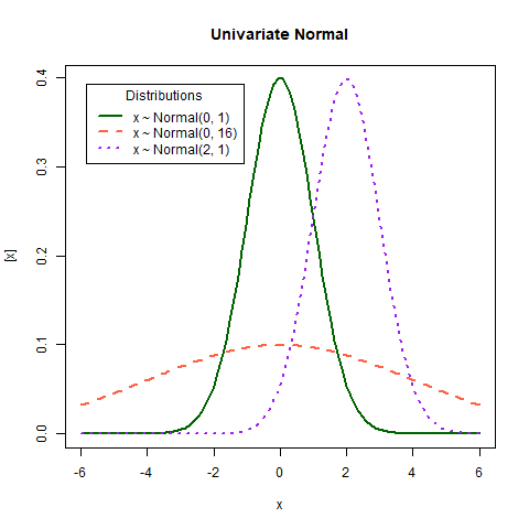
Discuss in the plot above:
- Expected value
- Variance
- Covariance?
On the covariance of two random variables \(y_1\) and \(y_2\)
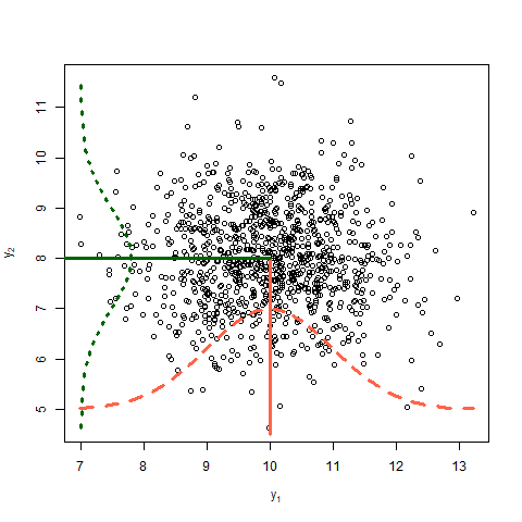
Covariance between two random variables means how the two random variables behave relative to each other. Essentially, it quantifies the relationship between their joint variability. The variance of a random variable is the covariance of a random variable with itself. Consider two variables \(y_1\) and \(y_2\) each with a variance of 1 and a covariance of 0.6. The data shown in Figure 4 arise from the multivariate normal distribution
\[\begin{bmatrix}y_1 \\ y_2 \end{bmatrix} \sim MVN \left( \begin{bmatrix} 10 \\ 8 \end{bmatrix} , \begin{bmatrix}1 & 0.6 \\ 0.6 & 1 \end{bmatrix} \right),\]where the means of \(y_1\) and \(y_2\) are 10 and 8, respectively, and their covariance structure is represented in the variance-covariance matrix. Remember,
\[\begin{bmatrix}y_1 \\ y_2 \end{bmatrix} \sim MVN \left( \begin{bmatrix} E(y_1) \\ E(y_2) \end{bmatrix} , \begin{bmatrix} Var(y_1) & Cov(y_1, y_2) \\ Cov(y_2,y_2) & Var(y_2) \end{bmatrix} \right).\]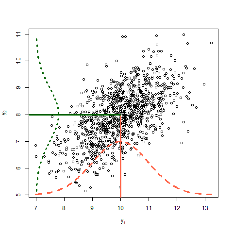
Discuss in the plot above:
- Expected value
- Variance
- Covariance
Adding a random effect to the model
The assumption behind independent observations
If we used the default model in most software written above, we would be assuming
\[\mathbf{y} \sim N(\boldsymbol{\mu}, \Sigma),\\ \begin{bmatrix}y_1 \\ y_2 \\ y_3 \\ y_4 \\ \vdots \\ y_n \end{bmatrix} \sim N \left( \begin{bmatrix}\mu_1 \\ \mu_2 \\ \mu_3 \\ \mu_4 \\ \vdots \\ \mu_n \end{bmatrix}, \sigma^2 \begin{bmatrix} 1 & 0 & 0 & 0 & \dots & 0 \\ 0 & 1 & 0 & 0 & \dots & 0 \\ 0 & 0 & 1 & 0 & \dots & 0 \\ 0 & 0 & 0 & 1 & \dots & 0 \\ \vdots & \vdots & \vdots & \vdots & \ddots & \vdots\\ 0 & 0 & 0 & 0 & \dots & 1 \end{bmatrix} \right),\]which is the same as
\[\begin{bmatrix}y_1 \\ y_2 \\ y_3 \\ y_4 \\ \vdots \\ y_n \end{bmatrix} \sim N \left( \begin{bmatrix}\mu_1 \\ \mu_2 \\ \mu_3 \\ \mu_4 \\ \vdots \\ \mu_n \end{bmatrix}, \begin{bmatrix} \sigma^2 & 0 & 0 & 0 & \dots & 0 \\ 0 & \sigma^2 & 0 & 0 & \dots & 0 \\ 0 & 0 & \sigma^2 & 0 & \dots & 0 \\ 0 & 0 & 0 & \sigma^2 & \dots & 0 \\ \vdots & \vdots & \vdots & \vdots & \ddots & \vdots\\ 0 & 0 & 0 & 0 & \dots & \sigma^2 \end{bmatrix} \right).\]Discuss the assumptions:
- Linearity
- Constant variance
- Independence
- Normality

Non-independent observations
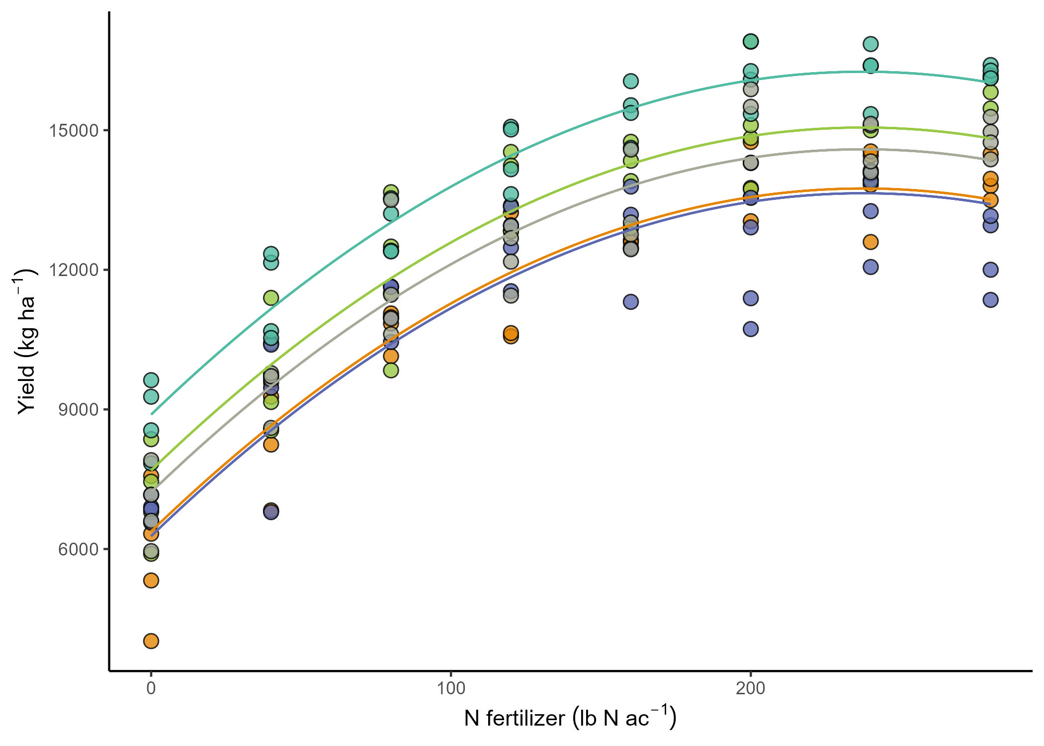
The yield data come from 5 different fields that were approximately homogeneous. Which means that the assumption of independence we made before was kind of a stretch. In reality, all observations from the same field have something in common. It’s not reasonable to assume that the observations are independent, because observations from the same field have more in common than observations from different fields. They share the soil and environments and, with that, a baseline fertility and yield potential.
Basically, we expect the yield response to N fertilizer is similar among fields, but the baseline (a.k.a., the intercept) to be field-specific. Then,
\[y_{ij} = \beta_{0j} + x_{ij} \beta_1 + \varepsilon_{ij}, \\ \varepsilon_{ij} \sim N(0, \sigma^2),\]Now, there are different ways to model that field-specific intercept.
How do we define \(\beta_{0j}\)?
This is a big forking path in statistical modeling. All-fixed models estimate the effects Mixed-effects models indicate what is similar to what via random effects.
Fixed effects
So far, we could have defined an all-fixed model,
\[y_{ij} = \beta_{0j} + x_{ij} \beta_1 + x^2_{ij} \beta_2 + \varepsilon_{ij}, \\ \beta_{0j} = \beta_0 + u_j \\ \varepsilon_{ij} \sim N(0, \sigma^2),\]where \(u_j\) is the effect of the \(j\)th field on the intercept (i.e., on the baseline). In this case, \(u_j\) is a fixed effect, which means it may be estimated via least squares estimation or maximum likelihood estimation. Under both least squares and maximum likelihood (assuming normal distribution), we may estimate the parameters by computing
\[\hat{\boldsymbol{\beta}}_{ML} = (\mathbf{X}^T\mathbf{X})^{-1}\mathbf{X}^T\mathbf{y},\]which yields the minimum variance unbiased estimate of \(\boldsymbol{\beta}\).
We still have \(\boldsymbol{\Sigma} = \begin{bmatrix} \sigma_{\varepsilon}^2 & 0 & 0 & 0 & \dots & 0 \\ 0 & \sigma_{\varepsilon}^2 & 0 & 0 & \dots & 0 \\ 0 & 0 & \sigma_{\varepsilon}^2 & 0 & \dots & 0 \\ 0 & 0 & 0 & \sigma_{\varepsilon}^2 & \dots & 0 \\ \vdots & \vdots & \vdots & \vdots & \ddots & \vdots\\ 0 & 0 & 0 & 0 & \dots & \sigma_{\varepsilon}^2 \end{bmatrix}\).
Random effects
We could also assume that the effects of the \(j\)th field (i.e., \(u_j\)) arise from a random distribution. The most common assumption (and the default in most statistical software) is that
\[u_j \sim N(0, \sigma^2_b).\]Now, we don’t estimate the effect, but the variance \(\sigma^2_b\).
Note that there are \(J\) levels of the random effects, meaning that a random effect is always categorical.
Also, now
where \(\mathbf{V} = Var(\mathbf{y})\) is the variance-covariance matrix of \(\mathbf{y}\), including residual variance and random-effects variance. Note that this formula yields the same point estimate for \(\boldsymbol{\beta}\), but with a different confidence interval.
Now, the variance-covariance matrix \(\boldsymbol{\Sigma}\) of the marginal distribution has changed (Figure 7). See next section for more details on how it’s changed.

Generalities on mixed models
Mixed models combine fixed effects and random effects. Generally speaking, we can write out a mixed-effects model using the model equation form, as
\[\mathbf{y} = \mathbf{X} \boldsymbol{\beta} + \mathbf{Z}\mathbf{u} + \boldsymbol{\varepsilon}, \\ \begin{bmatrix}\mathbf{u} \\ \boldsymbol{\varepsilon} \end{bmatrix} \sim \left( \begin{bmatrix}\boldsymbol{0} \\ \boldsymbol{0} \end{bmatrix}, \begin{bmatrix}\mathbf{G} & \boldsymbol{0} \\ \boldsymbol{0} & \mathbf{R} \end{bmatrix} \right),\]where \(\mathbf{y}\) is the observed response, \(\mathbf{X}\) is the matrix with the explanatory variables, \(\mathbf{Z}\) is the design matrix, \(\boldsymbol{\beta}\) is the vector containing the fixed-effects, \(\mathbf{u}\) is the vector containing the random effects, \(\boldsymbol{\varepsilon}\) is the vector containing the residuals, \(\mathbf{G}\) is the variance-covariance matrix of the random effects, and \(\mathbf{R}\) is the variance-covariance matrix of the residuals. Note that \(\mathbf{X} \boldsymbol{\beta}\) is the fixed effects part of the model, and \(\mathbf{Z}\mathbf{u}\) is the random effects part of the model.
Using the probability distribution form, we can then say that \(E(\mathbf{y}) = \mathbf{X}\boldsymbol{\beta}\) and \(Var(\mathbf{y}) = \mathbf{V} = \mathbf{Z}\mathbf{G}\mathbf{Z}' + \mathbf{R}\). Usually, we assume \(\mathbf{G} = \sigma^2_u \begin{bmatrix} 1 & 0 & 0 & \dots 0 \\ 0 & 1 & 0 & \dots & 0 \\ 0 & 0 & 1 & \dots & 0 \\ \vdots & \vdots & \vdots & \ddots & \vdots \\ 0 & 0 & 0 & \dots & 1 \end{bmatrix}\) and \(\mathbf{R} = \sigma^2 \begin{bmatrix} 1 & 0 & 0 & \dots & 0 \\ 0 & 1 & 0 & \dots & 0 \\ 0 & 0 & 1 & \dots & 0 \\ \vdots & \vdots & \vdots & \ddots & \vdots \\ 0 & 0 & 0 & \dots & 1 \end{bmatrix}\).
Then,
\[\mathbf{y} \sim N(\boldsymbol{\mu}, \Sigma),\] \[\Sigma = \begin{bmatrix} \sigma^2 + \sigma^2_u & \sigma^2_u & 0 & 0 & 0 & 0 &\dots & 0\\ \sigma^2_u & \sigma^2 + \sigma^2_u & 0 & 0 & 0 & 0 & \dots & 0 \\ 0 & 0 & \sigma^2 + \sigma^2_u & \sigma^2_u & 0 & 0 & \dots & 0 \\ 0 & 0 & \sigma^2_u & \sigma^2 + \sigma^2_u & 0 & 0 & \dots & 0 \\ 0 & 0 & 0 & 0 & \sigma^2 + \sigma^2_u & \sigma^2_u & \dots & 0 \\ 0 & 0 & 0 & 0 & \sigma^2_u & \sigma^2 + \sigma^2_u & \dots & \vdots \\ \vdots & \vdots & \vdots & \vdots & \vdots & \vdots & \ddots & \vdots \\ 0 & 0 & 0 & 0 & 0 & 0 & \dots & \sigma^2 + \sigma^2_u \end{bmatrix}.\]Take your time to digest the variance-covariance matrix above. What type of data do you think generated it?
Random effects
- By definition, random effects are regression coefficients that arise from a random distribution.
- Typically, a random effect \(u \sim N(0, \sigma^2_u)\).
- Note that this model for the parameter may result in shrinkage.
- We estimate the variance \(\sigma^2_u\).
- Calculating degrees of freedom can get much more complex than in all-fixed effects models (e.g., with unbalanced data, spatio-temporally correlated data, or non-normal data).
- In the context of designed experiments, random effects are assumed to be independent to each other and independent to the residual.
Estimation of parameters
“Estimation” is a term held mostly exclusive to fixed effects and variance components. Restricted maximum likelihood estimation (REML) is the default in most mixed effects models because, for small data (aka most experimental data), maximum likelihood (ML) provides variance estimates that are downward biased.
-
In REML, the likelihood is maximized after accounting for the model’s fixed effects.
- In ML, \(\ell_{ML}(\boldsymbol{\sigma; \boldsymbol{\beta}, \mathbf{y}}) = - (\frac{n}{2}) \log(2\pi)-(\frac{1}{2}) \log ( \vert \mathbf{V}(\boldsymbol\sigma) \vert ) - (\frac{1}{2}) (\mathbf{y}-\mathbf{X}\boldsymbol{\beta})^T[\mathbf{V}(\boldsymbol\sigma)]^{-1}(\mathbf{y}-\mathbf{X}\boldsymbol{\beta})\)
- In REML, \(\ell_{REML}(\boldsymbol{\sigma};\mathbf{y}) = - (\frac{n-p}{2}) \log (2\pi) - (\frac{1}{2}) \log ( \vert \mathbf{V}(\boldsymbol\sigma) \vert ) - (\frac{1}{2})log \left( \vert \mathbf{X}^T[\mathbf{V}(\boldsymbol\sigma)]^{-1}\mathbf{X} \vert \right) - (\frac{1}{2})\mathbf{r}[\mathbf{V}(\boldsymbol\sigma)]^{-1}\mathbf{r}\),
where \(p = rank(\mathbf{X})\), \(\mathbf{r} = \mathbf{y}-\mathbf{X}\hat{\boldsymbol{\beta}}_{ML}\).
- Start with initial values for \(\boldsymbol{\sigma}\), \(\tilde{\boldsymbol{\sigma}}\).
- Compute \(\mathbf{G}(\tilde{\boldsymbol{\sigma}})\) and \(\mathbf{R}(\tilde{\boldsymbol{\sigma}})\).
- Obtain \(\boldsymbol{\beta}\) and \(\mathbf{b}\).
- Update \(\tilde{\boldsymbol{\sigma}}\).
- Repeat until convergence.
Fixed effects versus random effects
What is behind a random effect:
- \[\hat{\boldsymbol{\beta}} \sim N \left( \boldsymbol{\beta}, (\mathbf{X}^T \mathbf{V}^{-1} \mathbf{X})^{-1} \right)\]
- \[u_j \sim N(0, \sigma^2_u)\]
- What process is being studied?
- How were the levels selected? (randomly, carefully selected)
- How many levels does the factor have, vs. how many did we observe?
- BLUEs versus BLUPs.
Read more in in Gelman (2005, page 20), “Analysis of variance—why it is more important than ever” [link], and Gelman and Hill (2006), page 245.
Group discussion: what determines if an effect should be random of fixed?
Case: scientists have decided they wanted to have 3 different environments (SE Kansas, NW Kansas, Central Kansas) for their experiments.
They design a randomized complete block design at each location.
However, they are not interested in studying the environments themselves.
How should they model the experiment?
Applied example
- Field experiment studying the effect of potassium on corn yield.
- One treatment factor: Potassium fertilizer (one-way treatment structure).
- Randomized Complete Block Design with 4 repetitions (design structure).
Building a statistical model
- What is the experiment blueprint? (aka design structure or structure in the data)
- What are the treatments?
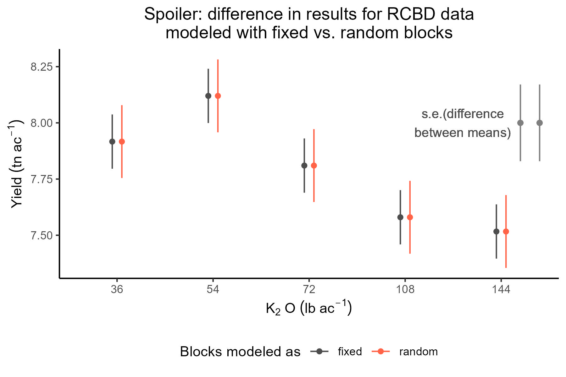
We can easily come up with two models:
- Blocks fixed \(y_{ijk} = \mu + \tau_i + \rho_j + \varepsilon_{ijk}; \ \ \varepsilon_{ijk} \sim N(0, \sigma^2)\).
- Blocks random \(y_{ijk} = \mu + \tau_i + u_j + \varepsilon_{ijk}; \ \ u_j \sim N(0, \sigma^2_u); \ \ \varepsilon_{ijk} \sim N(0, \sigma^2)\), where \(u\) and \(\varepsilon\) are independent.
library(lme4)
library(tidyverse)
library(emmeans)
library(latex2exp)

df <- read.csv("cochrancox_kfert.csv")
df$rep <- as.factor(df$rep)
df$K2O_lbac <- as.factor(df$K2O_lbac)
m_fixed <- lm(yield ~ K2O_lbac + rep, data = df)
m_random <- lmer(yield ~ K2O_lbac + (1|rep), data = df)

(mg_means_fixed <- emmeans(m_fixed, ~K2O_lbac, contr = list(c(1, 0, 0, 0, -1))))
## $emmeans
## K2O_lbac emmean SE df lower.CL upper.CL
## 36 7.92 0.121 8 7.64 8.19
## 54 8.12 0.121 8 7.84 8.40
## 72 7.81 0.121 8 7.53 8.09
## 108 7.58 0.121 8 7.30 7.86
## 144 7.52 0.121 8 7.24 7.79
##
## Results are averaged over the levels of: rep
## Confidence level used: 0.95
##
## $contrasts
## contrast estimate SE df t.ratio p.value
## c(1, 0, 0, 0, -1) 0.4 0.171 8 2.344 0.0471
##
## Results are averaged over the levels of: rep(mg_means_random <- emmeans(m_random, ~K2O_lbac, contr = list(c(1, 0, 0, 0, -1))))## $emmeans
## K2O_lbac emmean SE df lower.CL upper.CL
## 36 7.92 0.162 5.57 7.51 8.32
## 54 8.12 0.162 5.57 7.72 8.52
## 72 7.81 0.162 5.57 7.41 8.21
## 108 7.58 0.162 5.57 7.18 7.98
## 144 7.52 0.162 5.57 7.11 7.92
##
## Degrees-of-freedom method: kenward-roger
## Confidence level used: 0.95
##
## $contrasts
## contrast estimate SE df t.ratio p.value
## c(1, 0, 0, 0, -1) 0.4 0.171 8 2.344 0.0471
##
## Degrees-of-freedom method: kenward-roger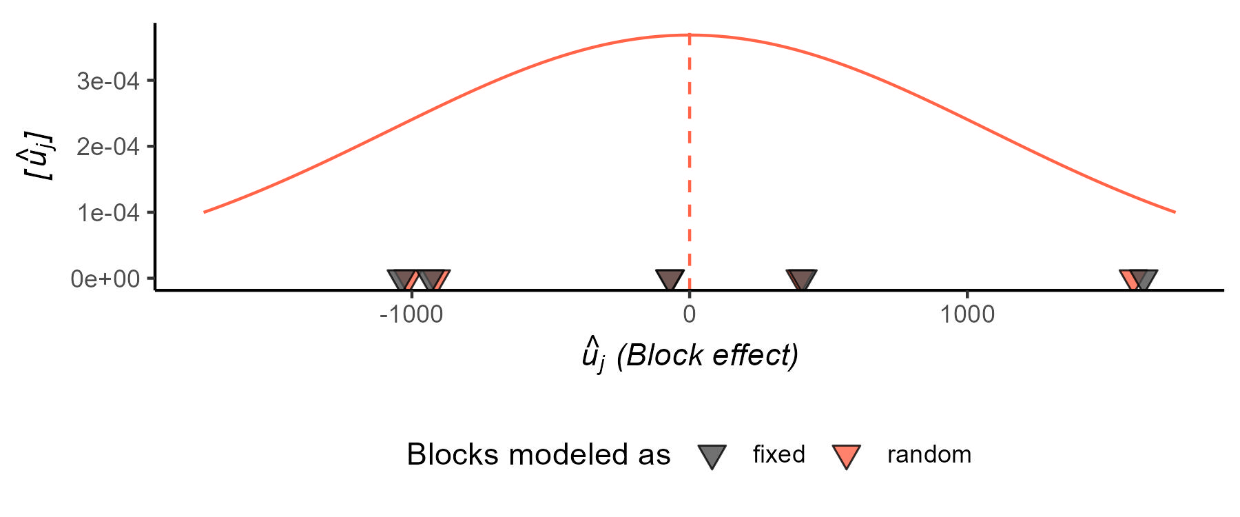
Discussions
Now we know what we mean when we say “factor A was considered fixed and factor B was considered random”!
Group discussion: What to write in the Materials and Methods section of a paper.
- Field-specific consensus
- Enough information to be reproducible
Example 1: A study to find out if water capture increased as the result of selection for yield in SX hybrids in the US corn-belt (Reyes et al., 2015). [link]

Example 2: A study to find out if developmental telomere attrition is a measure of state in birds, and hence should predict state-dependent decisions such as the relative value assigned to immediate versus delayed food rewards (Bateson et al., 2014). [link]
Summary
| Fixed effects | Random effects | |
|---|---|---|
| Where | Expected value | Variance-covariance matrix |
| Inference | Constant for all groups in the population of study | Differ from group to group |
| Usually used to model | Carefully selected treatments or genotypes | The study design (aka structure in the data, or what is similar to what) |
| Estimation | $$\hat{\boldsymbol{\beta}} \sim N \left( \boldsymbol{\beta}, (\mathbf{X}^T \mathbf{V}^{-1} \mathbf{X})^{-1} \right) $$ | $$u_j \sim N(0, \sigma^2_u)$$ |
| Method of estimation | Maximum likelihood, least squares. BLUEs. | Restricted maximum likelihood (shrinkage). BLUPs |
What’s next
- Linear mixed models applied to data generated by designed experiments.