Modeling data generated by designed experiments
Topics: Designed Experiments; Randomized Complete Block Designs; Split-Plot-Designs; Repeated Measures
Mixed-effects models combine fixed effects and random effects. Typically, we can define a Gaussian mixed-effects model as
\[\mathbf{y} = \mathbf{X} \boldsymbol{\beta} + \mathbf{Z}\mathbf{u} + \boldsymbol{\varepsilon}, \\ \begin{bmatrix}\mathbf{u} \\ \boldsymbol{\varepsilon} \end{bmatrix} \sim \left( \begin{bmatrix}\boldsymbol{0} \\ \boldsymbol{0} \end{bmatrix}, \begin{bmatrix}\mathbf{G} & \boldsymbol{0} \\ \boldsymbol{0} & \mathbf{R} \end{bmatrix} \right),\]where \(\mathbf{y}\) is the observed response,
\(\mathbf{X}\) is the matrix with the explanatory variables,
\(\mathbf{Z}\) is the design matrix,
\(\boldsymbol{\beta}\) is the vector containing the fixed-effects parameters,
\(\mathbf{u}\) is the vector containing the random effects parameters,
\(\boldsymbol{\varepsilon}\) is the vector containing the residuals,
\(\mathbf{G}\) is the variance-covariance matrix of the random effects,
and \(\mathbf{R}\) is the variance-covariance matrix of the residuals.
Typically, \(\mathbf{G} = \sigma^2_u \mathbf{I}\) and \(\mathbf{R} = \sigma^2 \mathbf{I}\).
If we do the math, we get that
Fixed effects versus random effects
| Fixed effects | Random effects | |
|---|---|---|
| Where | Expected value | Variance-covariance matrix |
| Inference | Constant for all groups in the population of study | Differ from group to group |
| Usually used to model | Carefully selected treatments or genotypes | The study design (aka structure in the data, or what is similar to what) |
| Assumptions | $$\hat{\boldsymbol{\beta}} \sim N \left( \boldsymbol{\beta}, (\mathbf{X}^T \mathbf{V}^{-1} \mathbf{X})^{-1} \right) $$ | $$u_j \sim N(0, \sigma^2_u)$$ |
| Method of estimation | Maximum likelihood, least squares | Restricted maximum likelihood (shrinkage) |
- Outline for this afternoon
- Designed experiments
- Applied examples
- Applied example I – RCBD
- Applied example II – Split-plot design (nested random effects)
- Applied example III – repeated measures
- Applied example IV – repeated measures with subsampling
- What’s next
Outline for this afternoon
- Review on designed experiments.
- Should blocks be fixed or random?
- Applications of increased complexity: random effects on the intercept, nested random effects, covariance functions (repeated measures).
Designed experiments
Golden Rules of designed experiments:
- Randomization
- Replication
- Local control
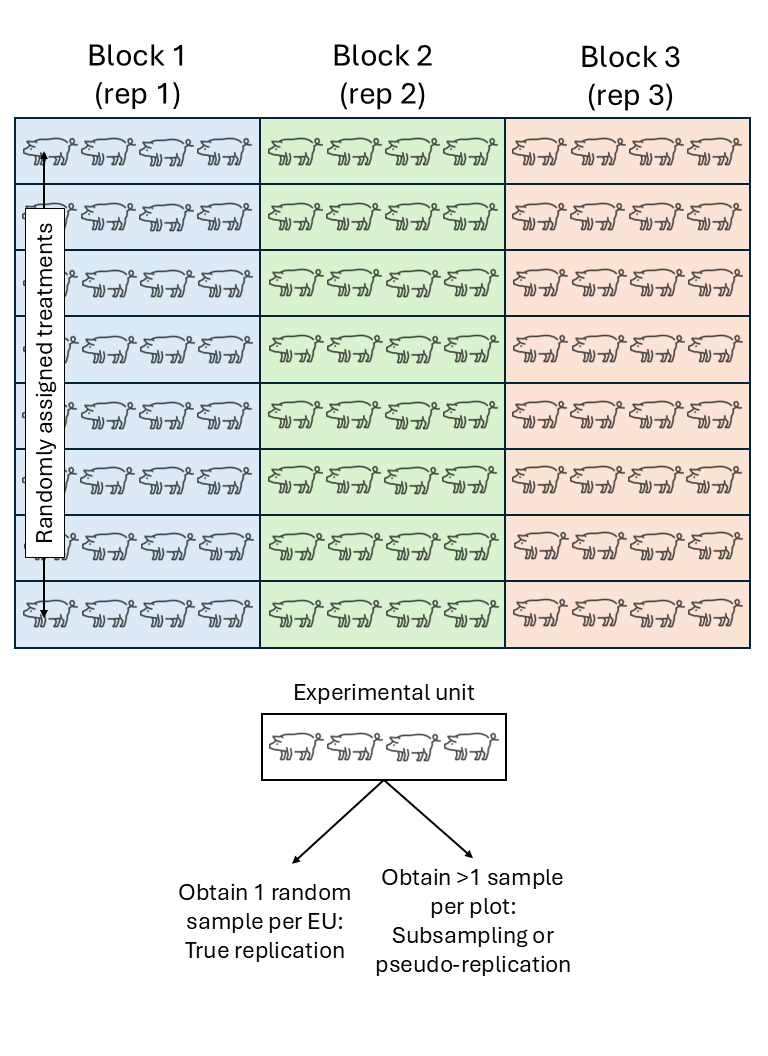
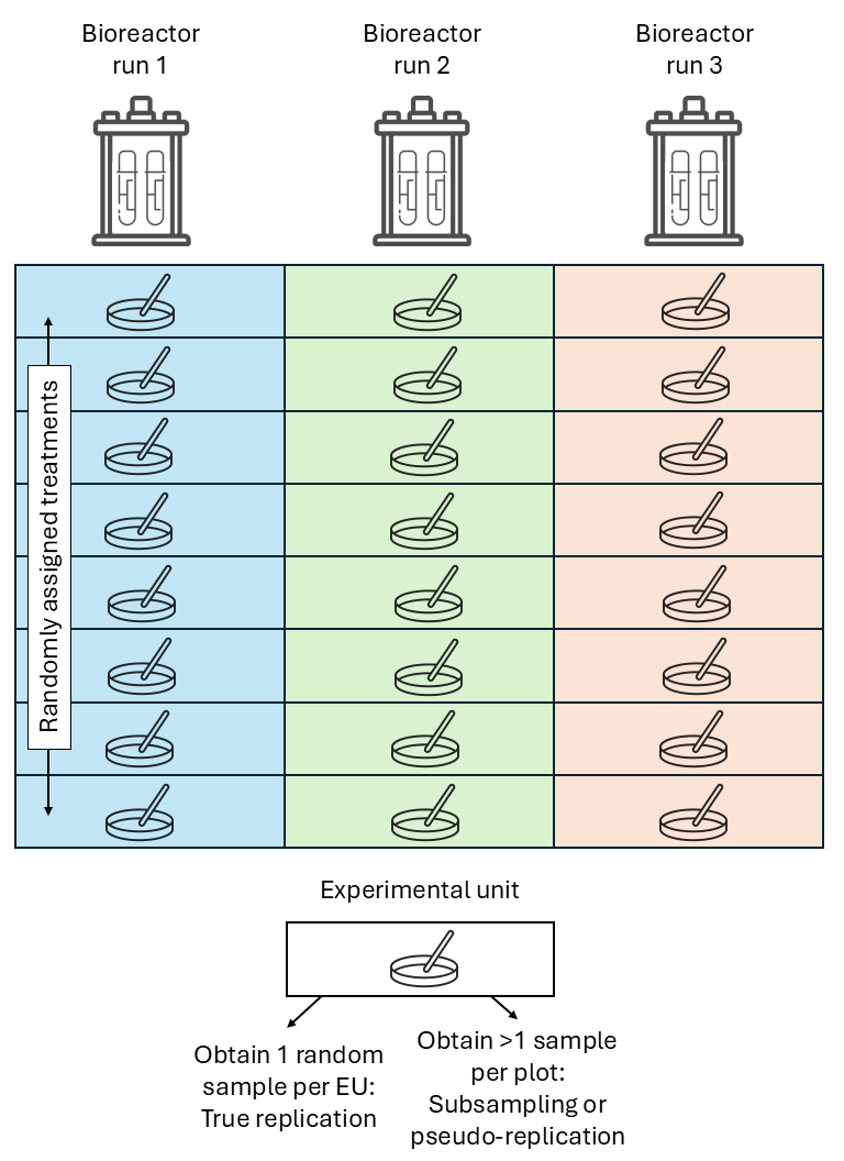
Experimental unit versus observational unit
- Experimental unit (EU): smallest entity to which a treatment is independently assigned.
- Observational unit (OU): entity on which observations are made.
- If OU \(>\) EU, not all observations are independent.
- The variance estimated from pseudoreplications (subsamples) is usually smaller than the variance estimated from true replications (experimental units).
Common types of designed experiments
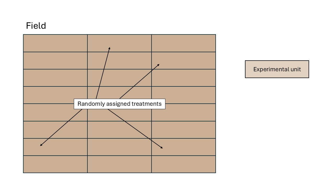
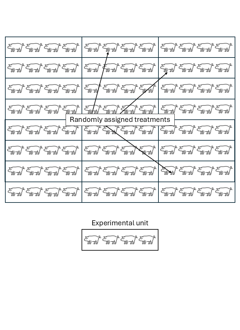
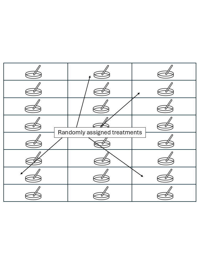
Completely Randomized Design (CRD)
We assume that all experimental units experienced similar conditions. In a field experiment setting, that means that all plots were located in an approximately homogeneous area. Observations are thus assumed independent to each other.
Statistical model the independent assumption seems reasonable, which is why we can keep the model where
\[y_{i} = \mu + \tau_i + \varepsilon_{i},\\ \varepsilon_{i} \sim N(0, \sigma^2).\]Let’s expand the variance-covariance matrix:
\[\Sigma = \begin{bmatrix} \sigma^2 & 0 & 0 & 0 & \dots & 0 \\ 0 & \sigma^2 & 0 & 0 & \dots & 0 \\ 0 & 0 & \sigma^2 & 0 & \dots & 0 \\ 0 & 0 & 0 & \sigma^2 & \dots & 0 \\ \vdots & \vdots & \vdots & \vdots & \ddots & \vdots\\ 0 & 0 & 0 & 0 & \dots & \sigma^2 \end{bmatrix}.\]Note that the elements in the off-diagonals are zeroes, because we are still keeping the assumption of independence (for now…).
Randomized complete block design (RCBD)
We assume that the experimental units did not experience similar conditions, but that an expert could determine groups of experimental units that did experience similar conditions. We call these groups of experimental units that experienced similar conditions “Blocks”. In a field experiment setting, that means that groups of plots were located in approximately homogeneous areas called blocks. In a study dealing with animals,this could be a repetition (i.e., a group of animals studied for the same timeframe). In a laboratory setting,this could be a day or a week where the scientists run the experiment.
All observations from the same block shared the same conditions and thus, shared a random effect for the intercept. Said common random effect for the intercept means that observations sharing a block are correlated. We can write out the statistical model
\[y_{ij} = \mu + \tau_i + u_j + \varepsilon_{ij},\\ u_{j} \sim N(0, \sigma^2_u), \\ \varepsilon_{ij} \sim N(0, \sigma^2),\]where \(y_{ijk}\) is the observation for the \(i\)th treatment in the \(j\)th block, \(\mu\) is the overall mean, \(\tau_i\) is the effect of the \(i\)th treatment, \(u_k\) is the random effect of the \(k\)th block, and \(\varepsilon_{ij}\) is the residual.
Assuming observations 1 to 10 belong to:
| Block | Treatment | Response |
|---|---|---|
| 1 | H | 16.8 |
| 1 | C | 14.02 |
| 1 | A | 11.37 |
| 1 | G | 12.30 |
| 1 | D | 12.1 |
| 1 | E | 12.04 |
| 1 | F | 14.5 |
| 1 | B | 9.8 |
| 2 | E | 10.5 |
| 2 | F | 14.1 |

Discussion I: Should blocks be fixed or random?
This discussion has been very controversial among applied statisticians.
| Blocks fixed | Blocks random | |
|---|---|---|
| What is being estimated | $$\hat{\boldsymbol{\beta}}_{b \times 1}$$ | $$\sigma^2_u$$ |
| Estimation cost in degrees of freedom | more | less |
| Point estimates | same | same |
| Standard error of treatment means | $$\sqrt{\frac{\sigma^2}{b}}$$ | $$\sqrt{\frac{\sigma^2 + \sigma^2_b}{b}}$$ |
| Standard error of mean differences | $$\sqrt{\frac{2\sigma^2}{b}}$$ | $$\sqrt{\frac{2\sigma^2}{b}}$$ |
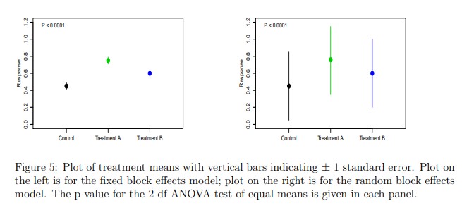
Check out Dixon (2016).
Discussion II: Should blocks be dropped if not significant?
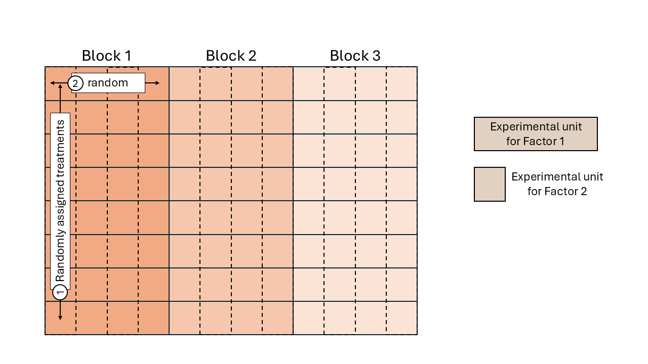
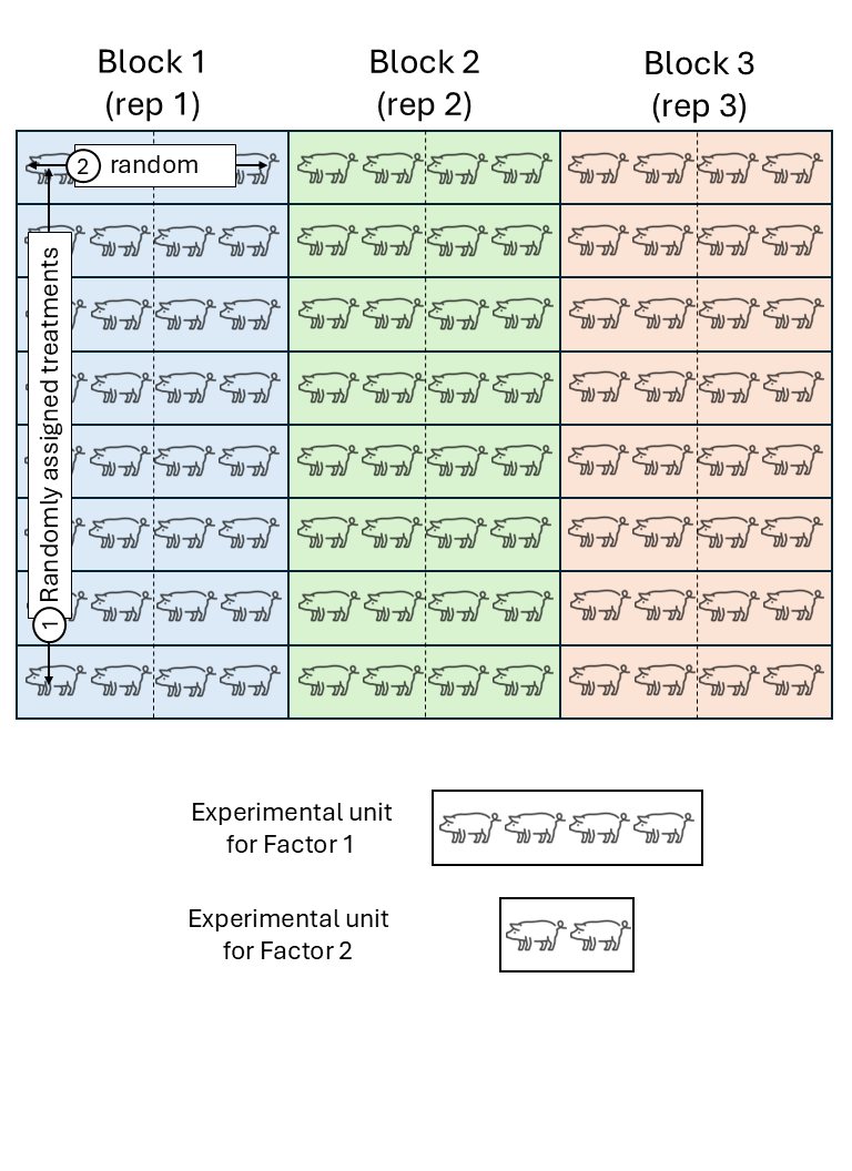
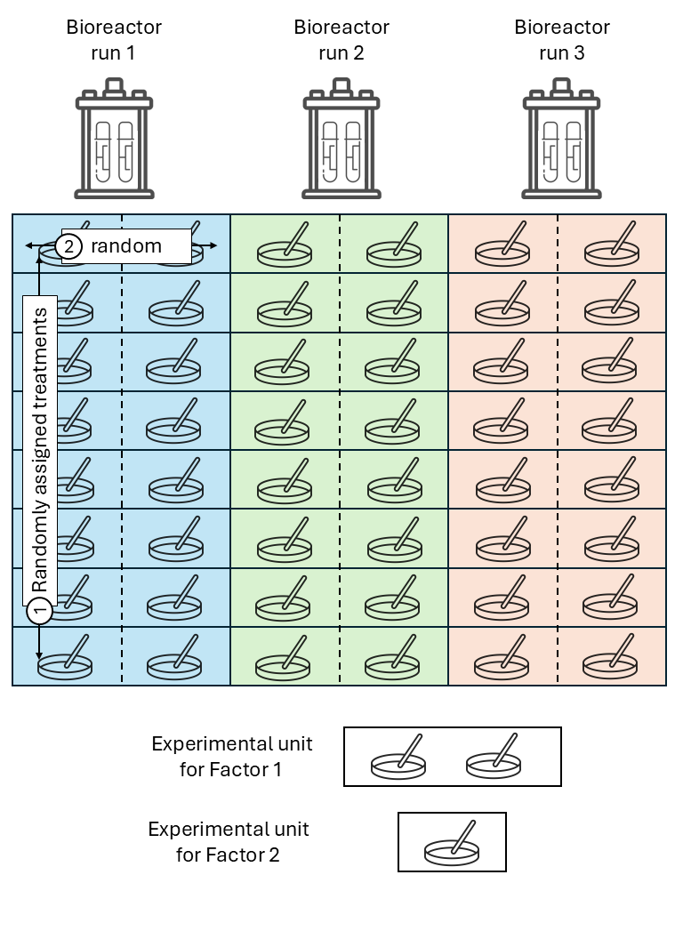
Split-plot design
Split-plot designs are hierarchical types of designs with at least two treatment factors, where the experimental unit for one treatment contains multiple experimental units of another treatment factor. The reason for this type of designs often go back to practical limitations for the application of some treatment factor (e.g., agricultural machinery that imposes the experimental unit size), making split-plot designs more convenient.
Treatments are randomized in a stepwise fashion:
- The levels of one treatment factor are randomly assigned to its experimental units (whole plots). In an RCBD, the treatments for the whole plots are randomly assigned within each block.
- Within the whole plots, the levels of the other treatment factor are randomly assigned to its experimental units (split plots), which are subsections of the whole plots. Note: we could think of the whole plots acting as “mini blocks” for the second treatment factor.
Again, all observations from the same block share the same random effect and are correlated.
Likewise, all observations from the same whole plot (\(\sim\)“mini block”) are correlated.
where \(y_{ijk}\) is the observation for the \(i\)th level of treatment factor 1, \(j\)th level of treatment factor 2, in the \(k\)th block, \(\mu\) is the overall mean, \(\tau_i\) is the main effect of the \(i\)th level of treatment factor 1, \(\alpha_j\) is the main effect of the \(j\)th level of treatment factor 2, \((\tau \alpha)_{ij}\) is their interaction, \(u_k\) is the random effect of the \(k\)th block, \(v_{i \vert k}\) is the random effect of the \(i\)th “miniblock” (whole plot) in the \(k\)th block, and \(\varepsilon_{ij}\) is the residual.
Assuming observations 1 to 4 belong to:
| Block | Treatment Factor 1 | Treatment Factor 2 | Response |
|---|---|---|---|
| 1 | H | a | 17.2 |
| 1 | H | c | 16.2 |
| 1 | H | b | 16.9 |
| 1 | H | d | 16.7 |
| 1 | C | d | 14.7 |
| 1 | C | c | 14.1 |
| 1 | C | b | 13.7 |
| 1 | C | a | 13.5 |
| 1 | A | c | 11.5 |
| 1 | A | d | 11.1 |
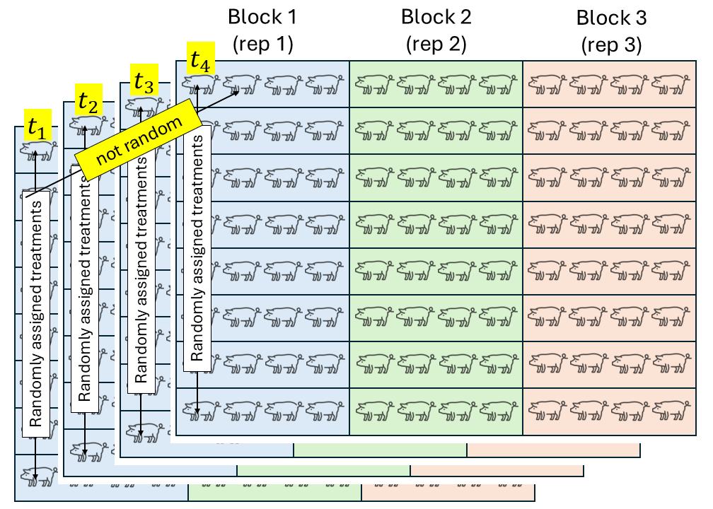
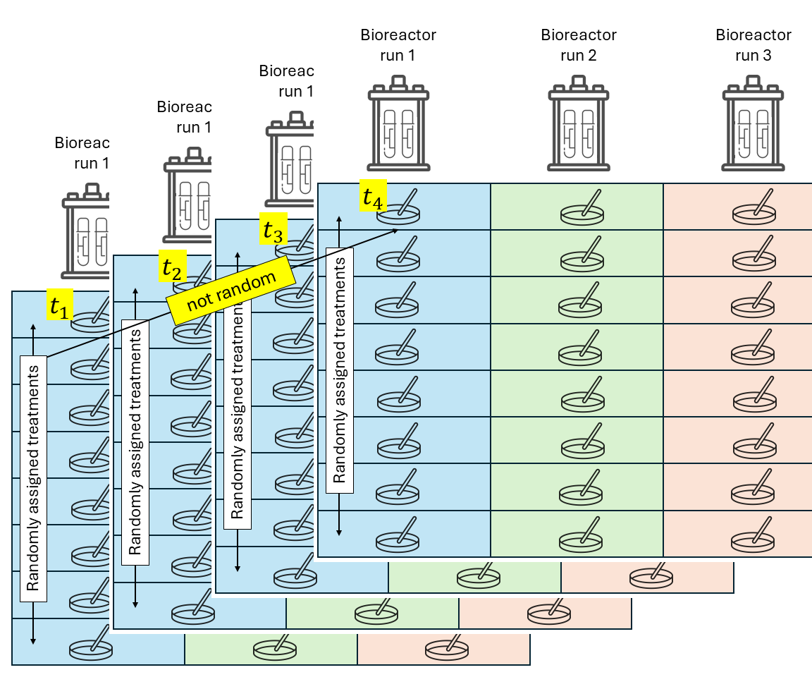
Repeated measures
Repeated measures designs are similar to split-plot desings, where time is at the subplot level. However, an important difference is that time cannot be randomly allocated, because it is unidirectional! The independence assumption does not hold and should be included in the model.
\[y_{ijkl} = \mu + \tau_i + \alpha_j + (\tau \alpha)_{ij} + u_{k} + v_{ijkl} + \varepsilon_{ijkl},\\ u_{k} \sim N(0, \sigma^2_u),\]where \(y_{ijk}\) is the observation for the \(i\)th treatment, \(j\)th time, in the \(k\)th block and the \(l\)th repetition within that block, \(\mu\) is the overall mean, \(\tau_i\) is the main effect of the \(i\)th level of treatment factor 1 (treatment), \(\alpha_j\) is the main effect of the \(j\)th level of treatment factor 2 (time), \((\tau \alpha)_{ij}\) is their interaction, \(u_k\) is the random effect of the \(k\)th block, \(v_{ijkl}\) is the random effect of the \(i\)th “miniblock” (whole plot) at the \(j\)th time, in the \(k\)th block and the \(l\)th repetition within that block, and \(\varepsilon_{ijkl}\) is the residual.
This time, unlike split-plots, \(v_{ijk} \nsim N(0, \sigma^2_v)\) because the treatment levels are not randomly assigned! Time is unidirectional and cannot be randomized. We can describe how different observations of a treatment \(i\) in block \(k\) are correlated, by looking at the distribution of \(\mathbf{v}_{ik}\):
\[\mathbf{v}_{ikl} \sim N(\boldsymbol{0}, \Sigma_{v, ik}), \\ \Sigma_{v, ik} = \sigma^2_v \begin{bmatrix} 1 & \rho & \rho^2 \\ \rho & 1 & \rho \\ \rho^2 & \rho & 1\end{bmatrix}.\]This example shows a first order autoregressive covariance structure. Other covariance functions include the compound symmetry covariance function, \(\mathbf{v}_{ikl} \sim N(\boldsymbol{0}, \Sigma_{v, ikl}), \\ \Sigma_{v, ikl} = \sigma^2_v \begin{bmatrix} 1 & \rho & \rho \\ \rho & 1 & \rho \\ \rho & \rho & 1\end{bmatrix}.\) and the unstructured covariance function, \(\mathbf{v}_{ikl} \sim N(\boldsymbol{0}, \Sigma_{v, ikl}), \\ \Sigma_{v, ikl} = \sigma^2_v \begin{bmatrix} 1 & \sigma^2_{12} & \sigma^2_{13} \\ \sigma^2_{21} & 1 & \sigma^2_{23} \\ \sigma^2_{31} & \sigma^2_{32} & 1\end{bmatrix}.\)
Note that we are still affecting the \(\mathbf{G}\) matrix, not the \(\mathbf{R}\) matrix – the residuals $\varepsilon_{ijk}$ are still iid normal. This difference may affect inference in non-normal responses (not the case yet), and is typically a modeling decision that should be carefully considered by the scientist. For other types of correlation functions and a discussion of the implications of G-side versus R-side correlations see Johnson and Milliken (2009), Stroup et al. (2024), and Muff et al. (2016).

Applied examples
Follow along with the R code here.
Applied example I - RCBD
The data below were generated by an experiment comparing sorghum genotypes (Omer et al., 2015). The data presented here correspond to a randomized complete block design ( design structure) that was performed to study different genotypes. Remember that blocks are assumed to be aproximately homogeneous within. A reasonable model, then, would be
\[y_{ij} = \mu + \tau_i + u_j + \varepsilon_{ij},\\ u_j \sim N(0, \sigma^2_u), \\ \varepsilon_{ij} \sim N(0, \sigma^2),\]where \(y_{ij}\) is the observed yield of the \(i\)th genotype in the \(j\)th block, \(\mu\) is the overall mean, \(\tau_i\) is the (fixed) effect of the \(i\)th genotype, \(u_j\) is the (random) effect of the \(j\)th block, \(\varepsilon_{ij}\) is the residual (i.e., the difference between predicted and observed) of the \(i\)th genotype in the \(j\)th block, \(\sigma^2_u\) is the variance among blocks, \(\sigma^2\) is the residual variance.
Since blocks are our only random effect, \(\mathbf{Z}\) can be defined as
\[\mathbf{Z} = \begin{array}{cc} \text{b}1 \ \ \text{b}2 \ \text{b}3 \ \ \text{b}4 \\ \begin{bmatrix} 1 & 0 & 0 & 0 \\ 1 & 0 & 0 & 0 \\ 1 & 0 & 0 & 0 \\ 1 & 0 & 0 & 0 \\ 0 & 1 & 0 & 0 \\ 0 & 1 & 0 & 0 \\ 0 & 1 & 0 & 0 \\ 0 & 1 & 0 & 0 \\ \vdots & \vdots & \vdots & \vdots \\ 0 & 0 & 0 & 1\end{bmatrix} \end{array}.\]Note that the matrix columns are labeled according to the block they are indicating.
If \(z_{ij} = 1\), that means that that observation (\(i\)th row) belongs to that block (\(j\)th column).
Otherwise, (i.e., \(z_{ij} = 0\)), that observation did not belong to that block.
library(glmmTMB)
library(agridat)
library(tidyverse)
library(DHARMa)

knitr::opts_chunk$set(fig.width=8, fig.height=4)

data(omer.sorghum)
dat <- omer.sorghum
dat <- dat %>%
  filter(env == "E3")

m_rcbd <- glmmTMB(yield ~ gen + (1|rep), data = dat)
## Formula:          yield ~ gen + (1 | rep)
## Data: dat
##       AIC       BIC    logLik  df.resid
##  958.9649 1004.4982 -459.4824        52
## Random-effects (co)variances:
##
## Conditional model:
##  Groups   Name        Std.Dev.
##  rep      (Intercept)  46.69
##  Residual             138.64
##
## Number of obs: 72 / Conditional model: rep, 4
##
## Dispersion estimate for gaussian family (sigma^2): 1.92e+04
##
## Fixed Effects:
##
## Conditional model:
## (Intercept)         gen1         gen2         gen3         gen4         gen5         gen6
##      671.15       -89.29      -155.81       133.78        78.11       -28.24      -356.50
##        gen7         gen8         gen9        gen10        gen11        gen12        gen13
##      265.91        70.23       142.01        67.37        56.99      -132.17       153.88
##       gen14        gen15        gen16        gen17
## -88.23 -24.57 -66.49 -385.95simulateResiduals(m_rcbd, plot = TRUE)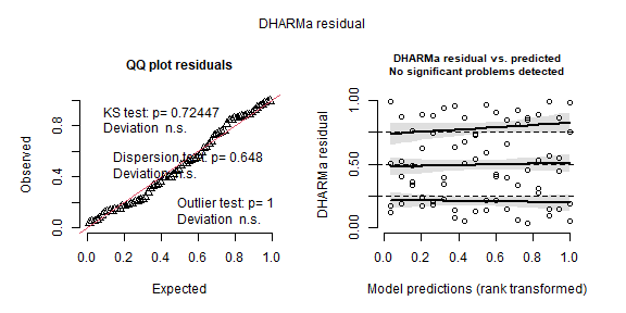
## Object of Class DHARMa with simulated residuals based on 250 simulations with refit = FALSE . See ?DHARMa::simulateResiduals for help.
##
## Scaled residual values: 0.208 0.336 0.04 0.06 0.868 0.876 0.864 0.848 0.532 0.904 0.964 0.624 0.996 0.944 0.728 0.136 0.992 0.984 0.184 0.492 ...car::Anova(m_rcbd)## Analysis of Deviance Table (Type II Wald chisquare tests)
##
## Response: yield
## Chisq Df Pr(>Chisq)
## gen 128.93 17 < 2.2e-16 ***
## ---
## Signif. codes: 0 '***' 0.001 '**' 0.01 '*' 0.05 '.' 0.1 ' ' 1marginal_means <- emmeans(m_rcbd, ~gen)
cld(marginal_means,
adjust = "sidak",
Letters = letters)## gen emmean SE df lower.CL upper.CL .group
## G17 285 73.1 52 56.1 514 a
## G06 315 73.1 52 85.5 544 a
## G02 515 73.1 52 286.2 744 ab
## G12 539 73.1 52 309.9 768 ab
## G01 582 73.1 52 352.7 811 abc
## G14 583 73.1 52 353.8 812 abc
## G16 605 73.1 52 375.5 834 abc
## G05 643 73.1 52 413.8 872 abc
## G15 647 73.1 52 417.5 876 abc
## G11 728 73.1 52 499.0 957 bcd
## G10 739 73.1 52 509.4 968 bcd
## G08 741 73.1 52 512.3 971 bcd
## G04 749 73.1 52 520.1 978 bcd
## G03 805 73.1 52 575.8 1034 bcd
## G09 813 73.1 52 584.0 1042 bcd
## G13 825 73.1 52 595.9 1054 bcd
## G07 937 73.1 52 707.9 1166 cd
## G18 1030 73.1 52 801.0 1259 d
##
## Confidence level used: 0.95
## Conf-level adjustment: sidak method for 18 estimates
## P value adjustment: sidak method for 153 tests
## significance level used: alpha = 0.05
## NOTE: If two or more means share the same grouping symbol,
## then we cannot show them to be different.
## But we also did not show them to be the same.Applied example II – Split-plot design (nested random effects)
This data example was first reported in Yates (1935). The data were generated by a split-plot experiment that was performed to study the yield of oats as affected by oat genotype (whole plot) and nitrogen fertilization (split plot).
\[y_{ijk} = \mu + \tau_i + \alpha_j +(\tau \alpha)_{ij} + u_k + v_{i \vert k} + \varepsilon_{ijk},\\ u_k \sim N(0, \sigma^2_u), \\ v_{i \vert k} \sim N(0, \sigma^2_v), \\ \varepsilon_{ijk} \sim N(0, \sigma^2),\]where \(y_{ijk}\) is the observed yield of the \(i\)th genotype and \(j\)th fertilizer treatment in the \(k\)th block, \(\mu\) is the overall mean, \(\tau_i\) is the (fixed) effect of the \(i\)th genotype, \(\alpha_j\) is the (fixed) effect of the \(j\)th fertilizer treatment, \((\tau \alpha)_{ij}\) is their interaction, \(u_k\) is the (random) effect of the \(k\)th block, \(v_{i \vert k}\) is the (random) effect of the \(i\)th whole plot (genotype) in the\(k\)th block, \(\varepsilon_{ijk}\) is the residual (i.e., the difference between predicted and observed) of the \(i\)th genotype and \(j\)th fertilizer treatment in the \(k\)th block, \(\sigma^2_u\) is the variance among blocks, \(\sigma^2_v\) is the variance among whole-plots, \(\sigma^2\) is the residual variance.
Now, the random effects are blocks and the whole plot (genotype)and thus, the matrix \(\mathbf{Z}\) gets bigger:
\[\mathbf{Z} = \begin{array}{cc} \text{b}1 \ \ \text{b}2 \ \ \text{b}3 \ \ \text{b}4 \ \ \text{b}5 \ \ \text{b}6 \ \text{g}1\text{b}1 \ \text{g}2\text{b}1 \dots \text{g}2\text{b}6 \\ \begin{bmatrix} 1 & 0 & 0 & 0 & 0 & 0 & 1 & 0 & \dots & 0\\ 1 & 0 & 0 & 0 & 0 & 0 & 0 & 1 & \dots & 0\\ 1 & 0 & 0 & 0 & 0 & 0 & 0 & 0 & \dots & 0\\ 1 & 0 & 0 & 0 & 0 & 0 & 0 & 0 & \dots & 0\\ 0 & 1 & 0 & 0 & 0 & 0 & 1 & 0 & \dots & 0\\ 0 & 1 & 0 & 0 & 0 & 0 & 0 & 1 & \dots & 0\\ 0 & 1 & 0 & 0 & 0 & 0 & 0 & 0 & \dots & 0\\ 0 & 1 & 0 & 0 & 0 & 0 & 0 & 0 & \dots & 0\\ \vdots & \vdots & \vdots & \vdots & \vdots & \vdots & \vdots & \vdots & \ddots & \vdots\\ 0 & 0 & 0 & 0 & 0 & 1 & 0 & 0 & \dots & 1 \end{bmatrix} \end{array}.\]dat <- yates.oats
dat$nf <- factor(dat$nitro)
m_splitplot <- glmmTMB(yield ~ gen*nf + (1|block/gen), data = dat)
summary(m_splitplot)## Family: gaussian ( identity )
## Formula: yield ~ gen * nf + (1 | block/gen)
## Data: dat
##
## AIC BIC logLik deviance df.resid
## 625.9 660.1 -298.0 595.9 57
##
## Random effects:
##
## Conditional model:
## Groups Name Variance Std.Dev.
## gen:block (Intercept) 88.38 9.401
## block (Intercept) 178.73 13.369
## Residual 147.57 12.148
## Number of obs: 72, groups: gen:block, 18; block, 6
##
## Dispersion estimate for gaussian family (sigma^2): 148
##
## Conditional model:
## Estimate Std. Error z value Pr(>|z|)
## (Intercept) 103.97216 6.06204 17.151 < 2e-16 ***
## gen1 0.52775 3.73090 0.141 0.8875
## gen2 5.81948 3.73090 1.560 0.1188
## nf1 -24.58331 2.47966 -9.914 < 2e-16 ***
## nf2 -5.08333 2.47966 -2.050 0.0404 *
## nf3 10.24998 2.47966 4.134 3.57e-05 ***
## gen1:nf1 0.08333 3.50677 0.024 0.9810
## gen2:nf1 1.45833 3.50677 0.416 0.6775
## gen1:nf2 -0.91668 3.50677 -0.261 0.7938
## gen2:nf2 3.79168 3.50677 1.081 0.2796
## gen1:nf3 -0.08331 3.50677 -0.024 0.9810
## gen2:nf3 -2.87502 3.50677 -0.820 0.4123
## ---
## Signif. codes: 0 '***' 0.001 '**' 0.01 '*' 0.05 '.' 0.1 ' ' 1simulateResiduals(m_splitplot, plot = TRUE)
## Object of Class DHARMa with simulated residuals based on 250 simulations with refit = FALSE . See ?DHARMa::simulateResiduals for help.
##
## Scaled residual values: 0.484 0.12 0.752 0.96 0.196 0.276 0.22 0.496 0.212 0.792 0.584 0.696 0.196 0.064 0.06 0.98 0.832 0.716 0.564 0.064 ...car::Anova(m_splitplot)## Analysis of Deviance Table (Type II Wald chisquare tests)
##
## Response: yield
## Chisq Df Pr(>Chisq)
## gen 3.5648 2 0.1682
## nf 135.6683 3 <2e-16 ***
## gen:nf 2.1803 6 0.9024
## ---
## Signif. codes: 0 '***' 0.001 '**' 0.01 '*' 0.05 '.' 0.1 ' ' 1marginal_means_splitplot <- emmeans(m_splitplot, ~gen:nf)cld(marginal_means_splitplot,
adjust = "sidak",
Letters = letters)## gen nf emmean SE df lower.CL upper.CL .group
## Victory 0 71.5 8.31 57 46.7 96.3 a
## GoldenRain 0 80.0 8.31 57 55.2 104.8 ab
## Marvellous 0 86.7 8.31 57 61.9 111.4 abc
## Victory 0.2 89.7 8.31 57 64.9 114.4 abcd
## GoldenRain 0.2 98.5 8.31 57 73.7 123.3 abcde
## Marvellous 0.2 108.5 8.31 57 83.7 133.3 bcdef
## Victory 0.4 110.8 8.31 57 86.1 135.6 bcdef
## GoldenRain 0.4 114.7 8.31 57 89.9 139.4 cdef
## Marvellous 0.4 117.2 8.31 57 92.4 141.9 def
## Victory 0.6 118.5 8.31 57 93.7 143.3 ef
## GoldenRain 0.6 124.8 8.31 57 100.1 149.6 f
## Marvellous 0.6 126.8 8.31 57 102.1 151.6 ef
##
## Confidence level used: 0.95
## Conf-level adjustment: sidak method for 12 estimates
## P value adjustment: sidak method for 66 tests
## significance level used: alpha = 0.05
## NOTE: If two or more means share the same grouping symbol,
## then we cannot show them to be different.
## But we also did not show them to be the same.Applied example III – repeated measures
One of our attendees kindly shared these data with us. The data were generated by an experiment that studied the effects of different feeding treatments on pigs. A total of 350 pigs were used in this study, with dietary treatment applied to each pen in a completely randomized design. Pig body temperature was measured at 5 points in time. The researchers wished to know if the feeding treatments affect body temperature.
\[y_{ijk} = \mu + \tau_i + \alpha_j + (\tau \alpha)_{ij} + u_{k} + v_{i j k} + \varepsilon_{ijk},\\ u_{k} \sim N(0, \sigma^2_u), \\ \varepsilon_{ijk} \sim N(0, \sigma^2),\]where \(y_{ij}\) is the observed temperature for the \(i\)th feed treatment,
in the \(k\)th pen,
on the \(j\)th day,
\(\mu\) is the overall mean,
\(\tau_i\) is the (fixed) effect of the \(i\)th feed treatment,
\(\alpha_j\) is the (fixed) effect of the \(j\)th day,
\((\tau \alpha)_{ij}\) is the interaction between the \(i\)th feed treatment and the \(j\)th day,
\(\varepsilon_{ijk}\) is the residual (i.e., the difference between predicted and observed) of the \(i\)th feed treatment,
in the \(k\)th pen,
on the \(j\)th day,
Note that we didn’t specify the distribution for \(v_{i j k}\). Normally we would have said \(v_{ijk} \sim N(0, \sigma^2_v)\), but now, the observations are not completely independent because they are following the same experimental unit through time. Assuming a first-order autoregressive structure, we can say
\[\mathbf{v}_{i k} \sim N(\boldsymbol{0}, \Sigma_{v,ik}), \\ \Sigma_{v,ik} = \sigma_v^2 \begin{bmatrix} 1 & \rho & \rho^2 & \rho^3 & \rho^4 \\ \rho & 1 & \rho & \rho^2 & \rho^3 \\ \rho^2 & \rho & 1 & \rho & \rho^2 \\ \rho^3 & \rho^2 & \rho & 1 & \rho \\ \rho^4 & \rho^3 & \rho^2 & \rho & 1 \end{bmatrix}.\]Note that in the code below we are using temperature in degrees Fahrenheit, because with Celsius it did not converge! More on troubleshooting in the Resources page.
options(contrasts = c("contr.treatment", "contr.poly"))

dd_temp$Pig <- as.factor(dd_temp$Pig)
dd_temp$Treatment <- as.factor(dd_temp$Treatment)
dd_temp$Pen <- as.factor(dd_temp$Pen)
dd_temp$Time <- as.factor(dd_temp$Time)
dd_temp$Temperature_F <- (dd_temp$Temperature_C *9/5) + 32

m_repeated <- glmmTMB(Temperature_C ~ Treatment * Time + ar1(1 + Time |Pen),
              family = gaussian(link = "identity"),
              data = dd_temp)
m_repeated <- glmmTMB(Temperature_F ~ Treatment * Time + ar1(1 + Time |Pen) ,
family = gaussian(link = "identity"),
data = dd_temp)res_repeated <- simulateResiduals(m_repeated, plot = TRUE)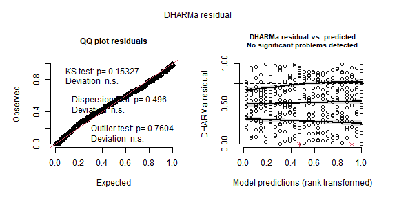
summary(m_repeated)## Family: gaussian ( identity )
## Formula: Temperature_F ~ Treatment * Time + ar1(1 + Time | Pen)
## Data: dd_temp
##
## AIC BIC logLik deviance df.resid
## 842.6 950.6 -393.3 786.6 322
##
## Random effects:
##
## Conditional model:
## Groups Name Variance Std.Dev. Corr
## Pen (Intercept) 0.2612 0.5111 0.55 (ar1)
## Residual 0.2545 0.5045
## Number of obs: 350, groups: Pen, 70
##
## Dispersion estimate for gaussian family (sigma^2): 0.255
##
## Conditional model:
## Estimate Std. Error z value Pr(>|z|)
## (Intercept) 1.037e+02 1.919e-01 540.2 < 2e-16 ***
## TreatmentB 2.286e-01 2.714e-01 0.8 0.399758
## TreatmentC 2.643e-01 2.714e-01 1.0 0.330235
## TreatmentD 1.357e-01 2.714e-01 0.5 0.617085
## TreatmentE 2.357e-01 2.714e-01 0.9 0.385195
## Time2 1.136e+00 2.346e-01 4.8 1.29e-06 ***
## Time4 1.086e+00 2.346e-01 4.6 3.68e-06 ***
## Time6 8.286e-01 2.346e-01 3.5 0.000412 ***
## Time12 2.357e-01 2.346e-01 1.0 0.314950
## TreatmentB:Time2 5.714e-02 3.317e-01 0.2 0.863239
## TreatmentC:Time2 3.357e-01 3.317e-01 1.0 0.311537
## TreatmentD:Time2 7.143e-01 3.317e-01 2.2 0.031302 *
## TreatmentE:Time2 -7.143e-02 3.317e-01 -0.2 0.829510
## TreatmentB:Time4 -5.643e-01 3.317e-01 -1.7 0.088935 .
## TreatmentC:Time4 3.571e-02 3.317e-01 0.1 0.914265
## TreatmentD:Time4 3.714e-01 3.317e-01 1.1 0.262855
## TreatmentE:Time4 -1.000e-01 3.317e-01 -0.3 0.763077
## TreatmentB:Time6 -2.357e-01 3.317e-01 -0.7 0.477366
## TreatmentC:Time6 9.286e-02 3.317e-01 0.3 0.779536
## TreatmentD:Time6 2.000e-01 3.317e-01 0.6 0.546565
## TreatmentE:Time6 -6.286e-01 3.317e-01 -1.9 0.058115 .
## TreatmentB:Time12 -1.071e-01 3.317e-01 -0.3 0.746711
## TreatmentC:Time12 8.571e-02 3.317e-01 0.3 0.796107
## TreatmentD:Time12 -2.190e-06 3.317e-01 0.0 0.999995
## TreatmentE:Time12 -3.857e-01 3.317e-01 -1.2 0.244935
## ---
## Signif. codes: 0 '***' 0.001 '**' 0.01 '*' 0.05 '.' 0.1 ' ' 1marginal_means_temp <- emmeans(m_repeated, ~ Treatment|Time)
cld(marginal_means_temp,
adjust = "sidak",
Letters = letters)## Time = 0:
## Treatment emmean SE df lower.CL upper.CL .group
## A 103.7 0.192 322 103.2 104.2 a
## D 103.8 0.192 322 103.3 104.3 a
## B 103.9 0.192 322 103.4 104.4 a
## E 103.9 0.192 322 103.4 104.4 a
## C 104.0 0.192 322 103.5 104.4 a
##
## Time = 2:
## Treatment emmean SE df lower.CL upper.CL .group
## A 104.8 0.276 322 104.1 105.5 a
## E 105.0 0.276 322 104.3 105.7 a
## B 105.1 0.276 322 104.4 105.8 a
## C 105.4 0.276 322 104.7 106.1 a
## D 105.7 0.276 322 105.0 106.4 a
##
## Time = 4:
## Treatment emmean SE df lower.CL upper.CL .group
## B 104.4 0.259 322 103.8 105.1 a
## A 104.8 0.259 322 104.1 105.4 a
## E 104.9 0.259 322 104.2 105.6 a
## C 105.1 0.259 322 104.4 105.7 a
## D 105.3 0.259 322 104.6 105.9 a
##
## Time = 6:
## Treatment emmean SE df lower.CL upper.CL .group
## E 104.1 0.249 322 103.5 104.8 a
## B 104.5 0.249 322 103.9 105.1 a
## A 104.5 0.249 322 103.9 105.2 a
## D 104.9 0.249 322 104.2 105.5 a
## C 104.9 0.249 322 104.2 105.5 a
##
## Time = 12:
## Treatment emmean SE df lower.CL upper.CL .group
## E 103.8 0.243 322 103.1 104.4 a
## A 103.9 0.243 322 103.3 104.5 a
## B 104.0 0.243 322 103.4 104.7 a
## D 104.1 0.243 322 103.4 104.7 a
## C 104.3 0.243 322 103.6 104.9 a
##
## Confidence level used: 0.95
## Conf-level adjustment: sidak method for 5 estimates
## P value adjustment: sidak method for 10 tests
## significance level used: alpha = 0.05
## NOTE: If two or more means share the same grouping symbol,
## then we cannot show them to be different.
## But we also did not show them to be the same.Applied example IV – repeated measures with subsampling
For this last example, one of our attendees kindly shared his data with us. The data were generated from an experiment that was studying the effect of different feed additives in swine production. A total of 300 pigs were used in this study, with dietary treatment applied to pen in a randomized complete block design.
- Experimental unit: pen.
- Observational unit: pig. 3 pigs per pen were sampled on day 5, 10, and 17 and fecal sample was then placed in drying oven at 55 C for 48 hours to determine fecal dry matter.
where \(y_{ijklm}\) is the observed fecal dry matter for the \(i\)th feed treatment, in \(j\)th day, \(k\)th room (\(\sim\) block) \(l\)th pen, and \(m\)th pig, \(\mu\) is the overall mean, \(\tau_i\) is the (fixed) effect of the \(i\)th feed treatment, \(\alpha_j\) is the (fixed) effect of the \(j\)th day, \((\tau \alpha)_{ij}\) is the interaction between the \(i\)th feed treatment and the \(j\)th day, \(u_k\) is the (random) effect of the \(k\)th room, \(v_{l \vert k}\) is the (random) effect of the \(l\)th pen in the \(k\)th room, \(\varepsilon_{ijklm}\) is the residual (i.e., the difference between predicted and observed) of the \(i\)th feed treatment, on the \(j\)th day, \(k\)th room (\(\sim\) block) \(l\)th pen, and \(m\)th pig, \(\sigma^2_u\) is the variance among rooms, \(\sigma^2_v\) is the variance among pens.
Note that we didn’t specify the distribution for \(w_{ijklm}\). Normally we would have said \(w_{ijklm} \sim N(0, \sigma^2_w)\), but now, the observations are not completely independent because they are following the same experimental unit through time. Assuming a first-order autoregressive structure, we say
\[\mathbf{w}_{i k lm} \sim N(\boldsymbol{\mu}, \Sigma_{w,ikl}), \\ \Sigma_{w,iklm} = \sigma^2_w \begin{bmatrix} 1 & \rho & \rho^2 \\ \rho & 1 & \rho \\ \rho^2 & \rho & 1\end{bmatrix}.\]dd_fecal <- read.csv("data/fecal_dm.csv")
dd_fecal$Pig <- as.factor(dd_fecal$Pig)
dd_fecal$Trt <- as.factor(dd_fecal$Trt)
dd_fecal$Room <- as.factor(dd_fecal$Room)
dd_fecal$Pen <- as.factor(dd_fecal$Pen)
dd_fecal$Day <- as.factor(dd_fecal$Day)
m_subsampling_repeated <- glmmTMB(dry_matter_perc ~ Trt * Day + ar1(1 + Day |Pig) + (1|Room/Pen),
data = dd_fecal)
res <- simulateResiduals(m_subsampling_repeated, plot = TRUE)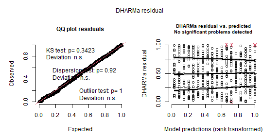
summary(m_subsampling_repeated)## Family: gaussian ( identity )
## Formula: dry_matter_perc ~ Trt * Day + ar1(1 + Day | Pig) + (1 | Room/Pen)
## Data: dd_fecal
##
## AIC BIC logLik deviance df.resid
## 3601.8 3700.6 -1777.9 3555.8 517
##
## Random effects:
##
## Conditional model:
## Groups Name Variance Std.Dev. Corr
## Pig (Intercept) 3.069620 1.75203 0.41 (ar1)
## Pen:Room (Intercept) 1.002794 1.00140
## Room (Intercept) 0.001016 0.03188
## Residual 35.916285 5.99302
## Number of obs: 540, groups: Pig, 180; Pen:Room, 60; Room, 2
##
## Dispersion estimate for gaussian family (sigma^2): 35.9
##
## Conditional model:
## Estimate Std. Error z value Pr(>|z|)
## (Intercept) 19.8414 1.1834 16.767 <2e-16 ***
## TrtB 3.8369 1.6732 2.293 0.0218 *
## TrtC 2.5830 1.6732 1.544 0.1227
## TrtD 1.5962 1.6732 0.954 0.3401
## TrtE 0.9596 1.6732 0.574 0.5663
## TrtF 2.3335 1.6732 1.395 0.1631
## Day10 -3.9525 1.5801 -2.501 0.0124 *
## Day17 -1.2710 1.5801 -0.804 0.4212
## TrtB:Day10 3.8430 2.2346 1.720 0.0855 .
## TrtC:Day10 -2.1745 2.2346 -0.973 0.3305
## TrtD:Day10 -2.1634 2.2346 -0.968 0.3330
## TrtE:Day10 -0.1957 2.2346 -0.088 0.9302
## TrtF:Day10 -4.5199 2.2346 -2.023 0.0431 *
## TrtB:Day17 -0.6552 2.2346 -0.293 0.7694
## TrtC:Day17 -2.8789 2.2346 -1.288 0.1976
## TrtD:Day17 -1.2935 2.2346 -0.579 0.5627
## TrtE:Day17 -0.4463 2.2346 -0.200 0.8417
## TrtF:Day17 -2.7244 2.2346 -1.219 0.2228
## ---
## Signif. codes: 0 '***' 0.001 '**' 0.01 '*' 0.05 '.' 0.1 ' ' 1marginal_means_feces <- emmeans(m_subsampling_repeated, ~ Day|Trt)
cld(marginal_means_feces,
adjust = "sidak",
Letters = letters)## Day = 5:
## Trt emmean SE df lower.CL upper.CL .group
## A 19.8 1.18 517 16.7 23.0 a
## E 20.8 1.18 517 17.7 23.9 a
## D 21.4 1.18 517 18.3 24.6 a
## F 22.2 1.18 517 19.0 25.3 a
## C 22.4 1.18 517 19.3 25.5 a
## B 23.7 1.18 517 20.6 26.8 a
##
## Day = 10:
## Trt emmean SE df lower.CL upper.CL .group
## F 13.7 1.26 517 10.4 17.0 a
## D 15.3 1.26 517 12.0 18.6 a
## A 15.9 1.26 517 12.6 19.2 a
## C 16.3 1.26 517 13.0 19.6 a
## E 16.7 1.26 517 13.3 20.0 a
## B 23.6 1.26 517 20.2 26.9 b
##
## Day = 17:
## Trt emmean SE df lower.CL upper.CL .group
## F 18.2 1.24 517 14.9 21.5 a
## C 18.3 1.24 517 15.0 21.5 a
## A 18.6 1.24 517 15.3 21.8 a
## D 18.9 1.24 517 15.6 22.1 a
## E 19.1 1.24 517 15.8 22.4 a
## B 21.8 1.24 517 18.5 25.0 a
##
## Confidence level used: 0.95
## Conf-level adjustment: sidak method for 6 estimates
## P value adjustment: sidak method for 15 tests
## significance level used: alpha = 0.05
## NOTE: If two or more means share the same grouping symbol,
## then we cannot show them to be different.
## But we also did not show them to be the same.What’s next
- Tomorrow, same time, same place.
- Non-normal response: proportions, counts, successes.
- If you’re not coming tomorrow: please answer this survey to help us improve future editions of the same workshop/create a follow-up based on demand.

Any questions? E-mail me!