Generalized linear mixed models

Topics: Non-normal data; Wrap-up

Outline for today

Distributions beyond the normal
Defining your generalized linear model
Applied examples
Workshop wrap-up: why mixed models are more important than ever.

What are GLMMs

Generalized Linear Models are models in which we can assume different distributions (from the exponential family) for our data beyond the Normal distribution.
Similar to general linear models, GLMs can also have random effects, thus, Generalized Linear Mixed Models - GLMMs.

The structure of a GLMM

Remember that for a LMMs, assuming \(\mathbf{y}\) arises from a normal distribution, we have:

\[\mathbf{y} =\mathbf{X}\boldsymbol{\beta} + \mathbf{Z}\mathbf{u} + \boldsymbol{\varepsilon} \\ \mathbf{\begin{bmatrix} \mathbf{u} \\ \boldsymbol{\varepsilon} \end{bmatrix} \sim \begin{pmatrix} \begin{bmatrix} 0 \\ 0 \end{bmatrix}, \begin{bmatrix} \mathbf{G} \; 0 \\ 0 \; \mathbf{R} \end{bmatrix} \end{pmatrix}}\]

In which:

\(\mathbf{X}\boldsymbol{\beta}\) represents our fixed part of the equation, where \(\mathbf{X}\) is a matrix informing the levels of our treatments and \(\boldsymbol{\beta}\) a vector containing the fixed-effects parameters.
\(\mathbf{Zu}\) represents our random part, where \(\mathbf{Z}\) is a matrix informing the levels of the random effects and \(\mathbf{u}\) is the vector containing the random effects parameters.
\(\boldsymbol{\varepsilon}\) is the vector containing the residuals.
From \(\mathbf{Zu} + \boldsymbol{\varepsilon}\) we have: \(\mathbf{G}\) is the variance-covariance matrix of the random effects, and \(\mathbf{R}\) is the variance-covariance matrix of the residuals.
- \(\mathbf{G} = \boldsymbol{\sigma^2_u}\mathbf{I}\) and \(\mathbf{R} = \boldsymbol{\sigma^2}\mathbf{I}\), in which \(\mathbf{I}\) is the identity matrix.

Which is similar to:

\[\mathbf{u} \sim N(0, \mathbf{I}\sigma^2_u) \\ \boldsymbol{\varepsilon} \sim N(0, \mathbf{I}\sigma^2)\]

In this case:

\[E(\mathbf{y}) = \mathbf{X}\boldsymbol{\beta}, \\ Var(\mathbf{y}) = \mathbf{ZGZ' + R}\]

We can also write this model as:

\[\mathbf{y} \sim N(\mathbf{X}\boldsymbol{\beta}, \; \mathbf{ZGZ' + R})\]

or:

\[\mathbf{y} \sim N(\mathbf{X}\boldsymbol{\beta}, \; \boldsymbol{\Sigma}) \\ \boldsymbol{\Sigma} = \mathbf{ZGZ' + R}\]

For GLMMs the structure changes based on the distribution we will assume for \(\mathbf{y}\), but is very similar to the last notation presented. A generic definition would be:

\[\mathbf{y|u} \sim P(\boldsymbol{\mu}, \; \phi)\]

Where:

\(\mathbf{y} \vert \mathbf{u}\) is the conditional distribution of the data \(y\), given any random effect \(u\),
\(\boldsymbol{\mu}\) is the expected value of \(\mathbf{y}\),
\(\phi\) is the dispersion parameter of the distribution,
the linear predictor of \(\mu\) is \(g(\mu) = \eta = \mathbf{X}\boldsymbol{\beta} + Zu\), where \(g(\cdot)\) is the link function that is applied to the expected value.

Components of GLMMs

Link Functions

Our linear predictor \(\mathbf{X}\boldsymbol{\beta}\) can produce all possible values in the y-axis of a plot, from \(- \; \infty\) to \(+ \; \infty\) depending on the value of the predictor variable. A link function links the linear predictor and the distribution assumed for the data \(\mathbf{y}\).

In the link scale, the mean of \(\mathbf{y}\) respect linearity of the linear predictor. In the response scale, the mean \(\mu\) is back transformed by the inverse link and respects the support of the distribution.

The link function is applied to the expected value (\(E(\mathbf{y})\)), and not to the observations. Transformation of the observations also effect the error, while link functions only affect the parameters controlling the expected value.

Example of link functions:

Link Function	Equation	Use	Why
Identity Link	\(g(\mu) = \mu\)	Normal dist.	\(E(y)\) can take any real value \((-\infty, \; +\infty)\)
Logit Link	\(g(\mu) = \log\left(\frac{\mu}{1-\mu}\right)\)	Logistic, Beta, Binomial dist.	\(E(y)\) can take any values between 0 and 1. Maps \((0, \; 1) \rightarrow (-\infty, \; +\infty)\)
Log Link	\(g(\mu) = \log(\mu)\)	Poisson, Gamma dist.	\(E(y)\) can take any positive values \((\mu > 0)\)

Log-transformations

Changes in the structure of the residuals: from normal to log-normal.
What is the target variable we aim to study?
If the data are not Gaussian, we must make them “act Gaussian”, essentially amounts to the modeling version of the “when you have a hammer, try to make every problem look like a nail” (Stroup et al., 2024, page 8).
No one-size-fits-all recommendation.

Distributional assumption for the data

GLMMs support different distributions from the exponential family. Distributions from the exponential family share common structure, but are relatively different among themselves.

What is an assumption?: Something you take as true about your data or about the process that generated it!

Important distributions to know are:

For continuous data: Normal, t, Gamma, Beta.
For discrete data: Binomial, Poisson, Negative Binomial.

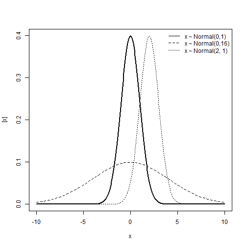
Normal distribution

\[y \sim N(\mu, \; \sigma^2)\] \[E(y) = \mu \\ Var(y) = \sigma^2\]

Support:

\[y \in (-\infty, \; +\infty)\]

Characteristics of the distribution

Type of variable: Continuous
Link: Identity, \(\eta = \mu\)
Mean and variance unrelated.

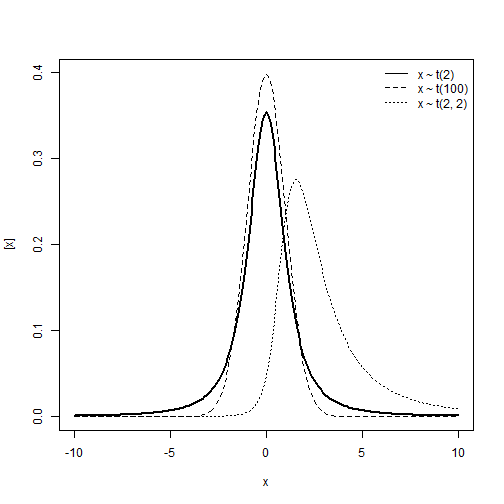
Student t distribution

\[y\sim t_{\nu}(\mu, \; \sigma^2)\] \[E(y) = \begin{cases} \mu, & \text{if } \nu > 1 \\ \text{undefined}, & \text{if } \text{else} \end{cases}\] \[Var(y) = \begin{cases} \frac{v}{v-2} \sigma^2, & \text{if } \nu > 2 \\ \text{undefined}, & \text{if } \text{else} \end{cases}\]

Support:

\[y \in (-\infty, \; +\infty)\]

Characteristics of the distribution

Type of variable: Continuous
Link: Identity, \(\eta = \mu\)
Mean and variance unrelated.

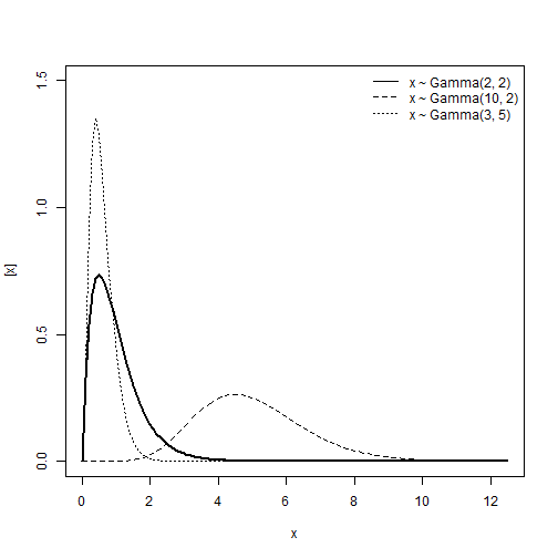
Gamma distribution

\[y \sim Gamma(\alpha, \; \beta)\] \[E(y) = \frac{\alpha}{\beta} \\ Var(y) = \frac{\alpha}{\beta^2}\]

Support:

\[y \in (0, \; +\infty)\]

Characteristics of the distribution

Type of variable: Continuous
Link: Log or Inverse, \(\eta = log(\mu)\) or \(\eta = \frac{1}{\mu}\)
If \(y \sim Gamma(\mu, \phi)\), the relationship between the mean and the variance is:
- Mean: \(\mu\)
- Var: \(\phi\mu^2\)

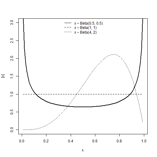
Beta distribution

\[y \sim Beta(\alpha, \; \beta)\] \[E(y) = \frac{\alpha}{\alpha + \beta} \\ Var(y) = \frac{\alpha\beta}{(\alpha+\beta)^2(\alpha+\beta+1)}\]

Support:

\[y \in (0, \; 1)\]

Characteristics of the distribution

Type of variable: Proportion
Link: Logit, \(\eta = logit(\mu) = log(\frac{\mu}{1-\mu})\)
If \(y \sim Beta(\mu, \phi)\):
- Mean: \(\mu\)
- Var: \(\frac{\mu(1-\mu)}{1+\phi}\)

Poisson distribution

\[y \sim Poisson(\lambda)\] \[E(y) = \lambda \\ Var(y) = \lambda\]

Support:

\[y \in (0, 1, 2, ..., +\infty)\]

Model the number of events occurring in a fixed interval of time/space given a rate of occurrence (\(\lambda\)).

Characteristics of the distribution

Type of variable: Discrete count
Link: Log, \(\eta = log(\lambda)\)
If \(y \sim Pois(\lambda)\):
- Mean: \(\lambda\)
- Var: \(\lambda\)

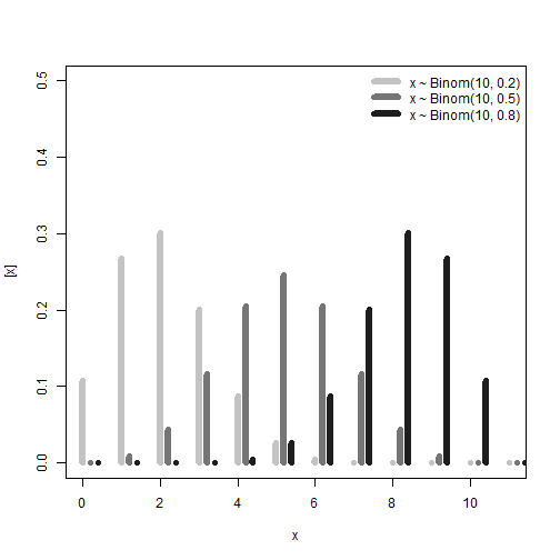
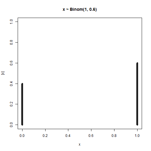
Binomial distribution

\[y \sim Binomial(n, p)\] \[E(y) = np \\ Var(y) = np(1-p)\]

Support:

\[y \in (0, 1, ..., n) \\ n \in (1, 2, ..., +\infty) \\ p \in (0, 1)\]

Model the number of successes in a fixed number of independent trials (\(n\)) with a given probability of success (\(p\)).

Characteristics of the distribution

Type of variable: Discrete or discrete proportion
Link: Logit or probit, \(\eta = log(\frac{p}{1-p})\) or \(\eta = \Phi^{-1}(p)\)
If \(y \sim Binomial(n, p)\):
- Mean: \(p = (np)/n\)
- Var: \(np(1-p)\)

Checkpoint:

Distributions beyond the normal
Defining your generalized linear model
Practical example

Working with GLMMs

Define a distribution that matches \(y\).
Define the linear predictor (fixed and random effects) \(\eta\).
Define the link function that connects \(E(y)\) of the assume distribution and the linear predictor \(\eta\).

Packages

library(agridat) # Agricultural datasets
library(glmmTMB) # Package to fit GLMMs
library(car) # Anova for mixed models
library(emmeans) # Extract marginal means
library(multcomp) # Mean multiple comparisons
library(DHARMa) # Model check

Example I - Disease Severity

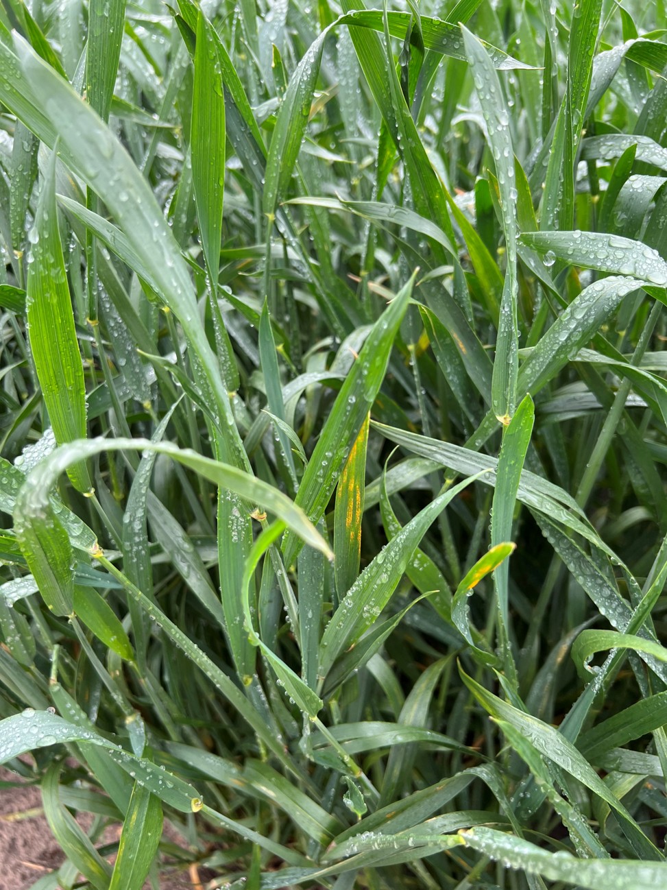
In this example we will evaluate disease severity. The data arises from a randomized complete block design experiment (RCBD) to test fungicide efficacy against yellow rust on wheat. The main response variable is disease severity. Severity refers to how much a specific organ is affected by a given disease. In this case it refers to the leaf area covered by yellow rust lesions, also know as pustules.

Data

head(d1)

##   fungicide block severity_o  severity
## 1         1     1   71.00000 0.7100000
## 2         1     2   75.33333 0.7533333
## 3         1     3   84.66667 0.8466667
## 4         1     4   71.00000 0.7100000
## 5         2     1   73.83333 0.7383333
## 6         2     2   60.66667 0.6066667

Define a distribution that matches \(y\).

\[y \sim Beta(\mu, \; \phi)\]

Why?
- Severity is a percentage: 0 - 100%, in proportion: 0 - 1.
- The support from the Beta distribution perfectly matches our response variable.
- Recall the support for the Beta distribution:

\[y \in (0, \; 1)\]

Define a linear predictor \(\eta\).

\[\eta_{ij} = \mu_0 + t_i + u_j\]

Where:
- \(\mu_0\) represents the overall/gran mean.
- \(t_i\) is the parameter for the effect of treatment, in this case, fungicides - Fixed effect.
- \(u_j\) is the parameter for the effect of block - Random effect.

Define the link function that connects \(E(y)\) of the assumed distribution and the linear predictor \(\eta\).

Logit link

\[g(\mu) = \eta = logit(\mu)\]

Why?
- Logit links \((-\infty, \; +\infty)\) to \((0, \; 1)\), that is our desired scale.

Model

\[y_{ij}|u_j \sim Beta(\mu_{ij}, \; \phi) \\ logit(\mu_{ij}) = \eta_{ij} = \mu_0 + t_i + u_j \\ u_j \sim N(0, \sigma^2_u)\]

Fitting the model

m1 <- glmmTMB(severity ~ fungicide + (1|block), family = beta_family(link = "logit"), data = d1)
summary(m1)

##  Family: beta  ( logit )
## Formula:          severity ~ fungicide + (1 | block)
## Data: d1
## 
##      AIC      BIC   logLik deviance df.resid 
##    -72.7    -46.5     50.4   -100.7       34 
## 
## Random effects:
## 
## Conditional model:
##  Groups Name        Variance  Std.Dev. 
##  block  (Intercept) 4.615e-10 2.148e-05
## Number of obs: 48, groups:  block, 4
## 
## Dispersion parameter for beta family (): 24.4 
## 
## Conditional model:
##             Estimate Std. Error z value Pr(>|z|)    
## (Intercept)   1.0975     0.2260   4.857 1.19e-06 ***
## fungicide2   -0.5546     0.3050  -1.819 0.068952 .  
## fungicide3   -0.8135     0.3018  -2.696 0.007020 ** 
## fungicide4   -0.7500     0.3024  -2.481 0.013118 *  
## fungicide5   -1.1663     0.3007  -3.878 0.000105 ***
## fungicide6   -2.7803     0.3478  -7.995 1.30e-15 ***
## fungicide7   -0.7072     0.3028  -2.335 0.019533 *  
## fungicide8   -0.9712     0.3008  -3.228 0.001245 ** 
## fungicide9   -1.6947     0.3063  -5.533 3.14e-08 ***
## fungicide10  -2.3778     0.3272  -7.267 3.68e-13 ***
## fungicide11  -3.2339     0.3787  -8.540  < 2e-16 ***
## fungicide12  -2.8120     0.3497  -8.042 8.85e-16 ***
## ---
## Signif. codes:  0 '***' 0.001 '**' 0.01 '*' 0.05 '.' 0.1 ' ' 1

Checking the model - Residuals

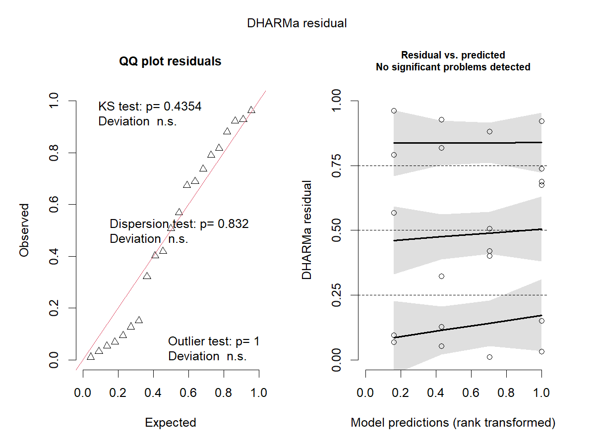
res_sim1 <- simulateResiduals(m1, plot = TRUE)

What are we checking here?

Residuals: “The footprint of the fitted model” - How much model predictions deviate from observations.

\[\epsilon_i = y_i - \hat{y}_i\]

For general linear mixed models our residuals are assumed to be normally distributed and with constant variance (\(\varepsilon \sim i.i.d. N(0, \; \sigma^2_\varepsilon)\)). In models with different distributional assumptions, residuals do not follow a known distribution, which makes it tricky to check models in a similar way we did before.

What is each test doing?

QQ-Plot
- Compare the quantiles¹ of two distributions, if they are similar, we expect them to fall on a one to one diagonal line. In this case, in the y-axis we have the quantiles of the simulated residuals and in the x-axis the quantiles of a standard uniform distribution.
- Kolmogorov-Smirnov test: Test for uniformity against a uniform distribution - \(Uniform(0, \; 1)\).
- Dispersion test: Variance in the observations vs. Variance on the simulations.
- Outlier test: Residual values of 0 or 1. Test if the number of outliers is appropriate to the size of the data. Does not quantify the amount of outliers.
Residual vs Predicted
- Show whether we have homocedasticity of the variances (constant variance across predicted values) or not. Usually, if higher or lower predicted values have higher or lower variance, the plot will present a “funnel” shape. Ideally the plot is a random scatter of points.
- Fit smoothed splines in three points of the quantile residuals, 0.25, 0.50, and 0.75. Test whether these lines are flat or have trends. For a random scatter, we do not expect to see trends at any of these points, this would indicate heterocedasticity.
- It also indicated when outliers are detected by producing a red asterisk.

ANOVA

Anova(m1)

## Analysis of Deviance Table (Type II Wald chisquare tests)
## 
## Response: severity
##            Chisq Df Pr(>Chisq)    
## fungicide 196.07 11  < 2.2e-16 ***
## ---
## Signif. codes:  0 '***' 0.001 '**' 0.01 '*' 0.05 '.' 0.1 ' ' 1

Post-hoc test - Mean comparisons

emmeans(m1, ~fungicide, type = "response")

##  fungicide response     SE  df asymp.LCL asymp.UCL
##  1            0.750 0.0424 Inf    0.6580     0.824
##  2            0.632 0.0477 Inf    0.5352     0.720
##  3            0.571 0.0490 Inf    0.4729     0.663
##  4            0.586 0.0488 Inf    0.4884     0.677
##  5            0.483 0.0495 Inf    0.3875     0.579
##  6            0.157 0.0348 Inf    0.0998     0.237
##  7            0.596 0.0486 Inf    0.4987     0.687
##  8            0.532 0.0495 Inf    0.4346     0.626
##  9            0.355 0.0473 Inf    0.2686     0.452
##  10           0.217 0.0402 Inf    0.1489     0.306
##  11           0.106 0.0286 Inf    0.0612     0.176
##  12           0.153 0.0344 Inf    0.0966     0.233
## 
## Confidence level used: 0.95 
## Intervals are back-transformed from the logit scale

What if we use a less appropriate assumption for severity?

Let’s check Gamma!

m1_2 <- glmmTMB(severity_o ~ fungicide + (1|block), family = Gamma(link = "log"), data = d1)
res_sim1_2 <- simulateResiduals(m1_2, plot = TRUE)

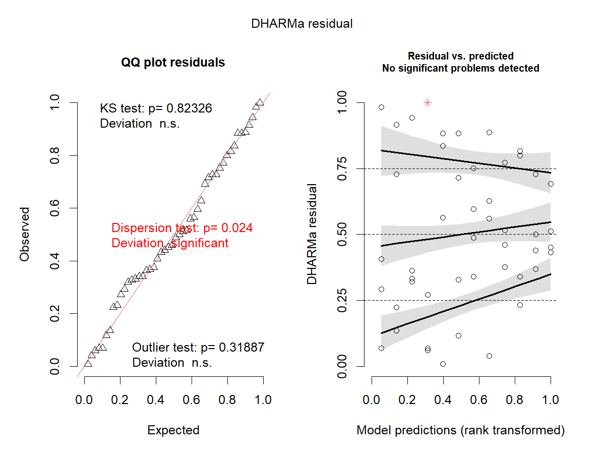
Recall:

Gamma - \(Var(y) = \phi\mu^2\)
Beta - \(Var(y) = \frac{\mu(1-\mu)}{1+\phi}\)

Dispersion on the Beta model

disp1 <- testDispersion(m1)

Dispersion on the Gamma model

disp1_2 <- testDispersion(m1_2)

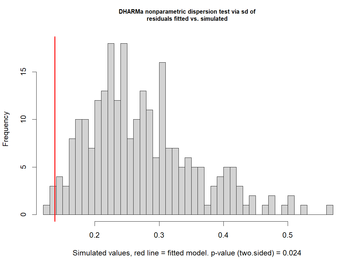
Signs of underdispersion

Dispersion: How spread out the data are around their mean - Relationship between the variance and the mean assumed by the distribution in the GLMM.

Underdispersion: The dispersion in the observed data is lower than the one expected by the model
Overdispersion: The dispersion in the observed data is higher than the one expected by the model

Example 2 - Seed germination

The following data arise from an experiment studying germination of Orobanche seeds (Crowder, 1978).
The data indicate the total number of seeds (\(n\)) and the number of germinated seeds (\(germ\)). The experiment was conducted as a completely randomized design with a 2 x 2 factorial treatment structure for type of extract (bean or cucumber) and extract concentration (o75 and o73).

Data

head(d2)

##   plate gen extract germ  n
## 1    P1 O75    bean   10 39
## 2    P2 O75    bean   23 62
## 3    P3 O75    bean   23 81
## 4    P4 O75    bean   26 51
## 5    P5 O75    bean   17 39
## 6    P6 O73    bean    8 16

Define a distribution that matches \(y\).

\[y \sim Binomial(n, \; p)\]

Why?
- We have the number of trials \(n\)
- For each trial we have the number of successes \(germ\)
- Remember the support for the Binomial distribution:

\[y \in (1, 2, ..., n)\]

Define a linear predictor \(\eta\).

\[\eta_{ij} = \mu_0 + ex_i + gen_j + (ex \times gen)_{ij}\]

Where:
- \(\mu_0\) represents the overall/gran mean.
- \(ex_i\) is the parameter for the effect of extract - Fixed effect.
- \(gen_j\) is the parameter for the effect of dilution - Fixed effect.
- \((ex \times gen)_{ij}\) is the parameter for the effect of the interaction between the extract and the dilution.

Define the link function that connects \(E(y)\) of the assume distribution and the linear predictor \(\eta\).

Logit link

\[g(p) = \eta = logit(p)\]

Why?
- Logit links \((-\infty, \; +\infty)\) to \((0, \; 1)\), that is our desired scale.

Model

\[y_{ij} \sim Binomial(n, \; p) \\ logit(p) = \eta_{ij} = \mu_0 + ex_i + gen_j + (ex \times gen)_{ij}\]

Fitting the model

m2 <- glmmTMB(cbind(germ, n-germ) ~ extract*gen, family = binomial(link = "logit"), data = d2)
summary(m2)

##  Family: binomial  ( logit )
## Formula:          cbind(germ, n - germ) ~ extract * gen
## Data: d2
## 
##      AIC      BIC   logLik deviance df.resid 
##    117.9    122.1    -54.9    109.9       17 
## 
## 
## Conditional model:
##                        Estimate Std. Error z value Pr(>|z|)  
## (Intercept)             -0.4122     0.1842  -2.238   0.0252 *
## extractcucumber          0.5401     0.2498   2.162   0.0306 *
## genO75                  -0.1459     0.2232  -0.654   0.5132  
## extractcucumber:genO75   0.7781     0.3064   2.539   0.0111 *
## ---
## Signif. codes:  0 '***' 0.001 '**' 0.01 '*' 0.05 '.' 0.1 ' ' 1

Different ways to fit the model with Binomial distribution – depends on what you have.
- Important point: Remember what we are modeling - Probability of success: \(p\).
- For Binomial distribution:
  - Case 1: \(y\) = Counts of success with known trials - Success and Failures = (success, trials - success).
  - Case 2: \(y\) = Counts of successes with weights - success/trials and weights = trials.
    - Only if proportions come from counts!
  - Case 3: A special case: \(y\) = Binary outcomes (0/1 per observation) - Binomial with n = 1 - Logistic regression.
- For Beta distribution:
  - Case 4: \(y\) = Proportions not from counts (between 0 and 1) - No trial number, proportion only
    - Do not use Binomial distribution here!

# Case 1
glmmTMB(cbind(germ, n-germ) ~ extract*gen, family = binomial(link = "logit"), data = data)

# Case 2
glmmTMB(germ/n ~ extract*gen, family = binomial(link = "logit"), weights = n, data = data)

# Case 3 - If germinated = yes (1) / no (0)
glmmTMB(germinated ~ extract*gen, family = binomial(link = "logit"), data = data)

# Case 4 - From example 1 - Severity: Proportion of area damaged by disease
glmmTMB(severity ~ fungicide + (1|block), family = beta_family(link = "logit"), data = data)

For the logistic regression:

Checking the model

res_sim2 <- simulateResiduals(m2, plot = TRUE)

ANOVA

Anova(m2)

## Analysis of Deviance Table (Type II Wald chisquare tests)
## 
## Response: cbind(germ, n - germ)
##               Chisq Df Pr(>Chisq)    
## extract     53.3974  1  2.725e-13 ***
## gen          3.0426  1    0.08111 .  
## extract:gen  6.4477  1    0.01111 *  
## ---
## Signif. codes:  0 '***' 0.001 '**' 0.01 '*' 0.05 '.' 0.1 ' ' 1

Marginal means

emmeans(m2, ~extract*gen, type = "response")

##  extract  gen  prob     SE  df asymp.LCL asymp.UCL
##  bean     O73 0.398 0.0441 Inf     0.316     0.487
##  cucumber O73 0.532 0.0420 Inf     0.449     0.613
##  bean     O75 0.364 0.0292 Inf     0.309     0.423
##  cucumber O75 0.681 0.0271 Inf     0.626     0.732
## 
## Confidence level used: 0.95 
## Intervals are back-transformed from the logit scale

Workshop wrapup - Hierarchical models

Why are mixed models sometimes called ‘hierarchical’ or ‘multilevel’ models?

What is an hierarchical model?

\[y_{ij}|u_j \sim N(\mu_{ij}, \; \sigma^2) \\ \mu_{ij} = \eta_{ij} = \mu_0 + t_i + u_j \\ u_j \sim N(0, \sigma^2_u)\]

Data model: The conditional distribution we are assuming for \(y\).

\[y_{ij}|u_j \sim N(\mu_{ij}, \; \sigma^2)\]

Process model: The functions that shapes the expected value/mean \(\mu\), and the link function connecting it to the boundaries of the assumed distribution - Processes generating the data.

\[\mu_{ij} = \eta_{ij} = \mu_0 + t_i + u_j\]

Parameter model: The random effects structure, the distribution of the random effects that capture the variation among groups.

\[u_j \sim N(0, \; \sigma_u^2)\]

But what else is in here?

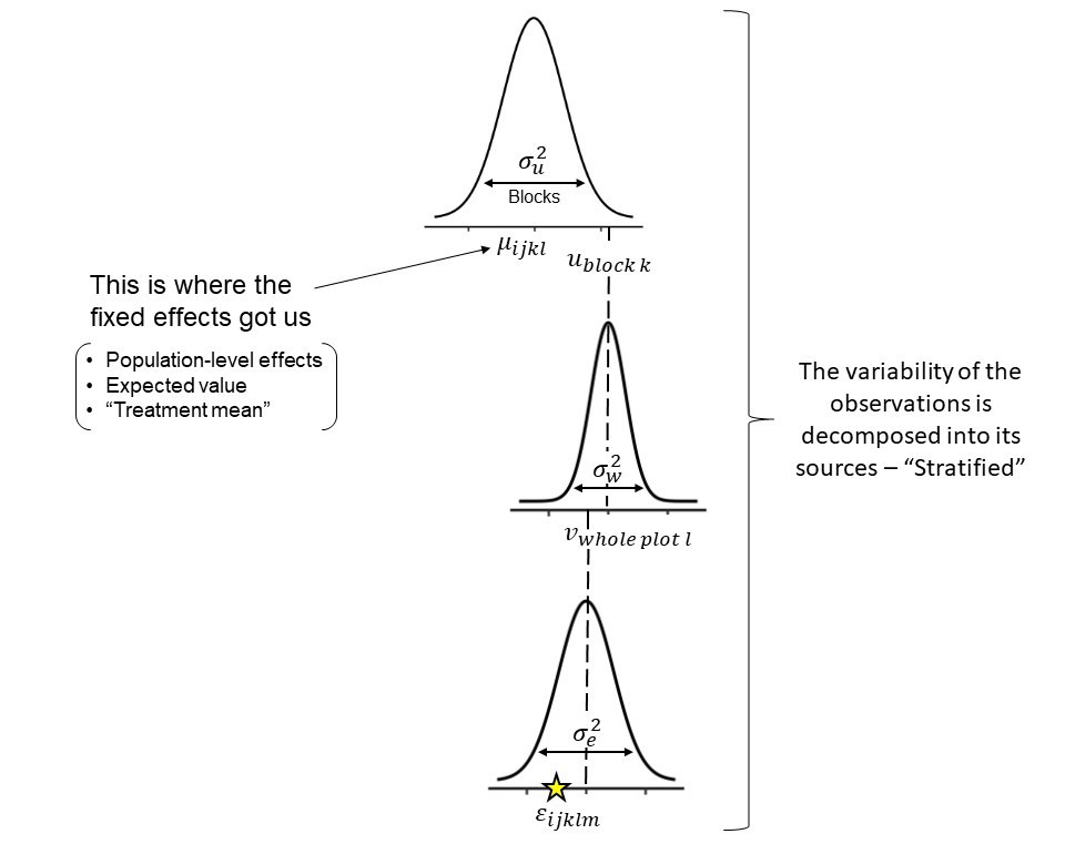
Let’s consider a split-plot design example: Stratification of random effects - Different levels structured

The model:

\[y_{ijkl}|u_k, \; w_l \sim N(\mu_{ijkl}, \; \sigma^2) \\ \mu_{ijkl} = \eta_{ijkl} = \mu_0 + f_i + v_j + u_k + w_l \\ u_k \sim N(0, \; \sigma_u^2) \\ w_l \sim N(0, \; \sigma_w^2)\]

Where:

\(\mu_0\) is the overall mean.
\(f_i\) is the fixed effect of fungicide applied to the whole plot.
\(v_j\) is the fixed effect of variety applied to the subplot level.
\(u_k\) is the random effect of the block.
\(w_l\) is the random effect of the whole plot level, that comes from \(u_k*f_i\).
The subplot level is nested with residuals, which is parametrized by \(\sigma^2\).

Major benefits we get from mixed models

Information is shared across groups
More robust under unbalanced scenarios
Very helpful to handle missing data
No need to average across observations - information is preserved!

I want to convince the reader of something that appears unreasonable: multilevel regression deserves to be the default form of regression. Papers that do not use multilevel models should have to justify not using a multilevel approach. Certainly some data and contexts do not need the multilevel treatment. But most contemporary studies in the social and natural sciences, whether experimental or not, would benefit from it. Perhaps the most important reason is that even well-controlled treatments interact with unmeasured aspects of the individuals, groups, or populations studied. This leads to variation in treatment effects, in which individuals or groups vary in how they respond to the same circumstance. Multilevel models attempt to quantify the extent of this variation, as well as identify which units in the data responded in which ways.

–Statistical Rethinking, Richard McElreath.

[Also see McEreath’s blog post]

What’s next

Check out the books in the Resources tab.
We will be repeating this workshop in the future! Tell your friends and family!
Claudio will be teaching a workshop on applied Bayesian modeling next Spring (2026).
Josefina will be teaching STAT 720 next Summer (2026) and STAT 870 next Fall.
Feel free to reach out with questions/concerns/more advanced questions.
Please answer this survey to help us improve future editions of the same workshop/create a follow-up based on demand.

References

Quantiles divide a dataset into equal-sized subsets, helping to understand more about the distribution of the data. ↩